The automobile market in Ukraine represents a typical case of international oligopolistic set-up. The theoretical modelling of international oligopoly dates back to the work of Dixit (1984). Although simple, his framework enables to determine major differences between the cases of perfect competition and oligopoly for trade policy. A more general study of Eaton and Grossman (1986) continues the development aimed at a rigorous modelling of international oligopoly under different assumptions about the nature of competition. Cheng (1988) further develops the approach pioneered by Eaton and Grossman, and in particular elaborates the case of domestic consumption of goods produced by international oligopoly. In the following discussion I’ll try to extend the methodology of Cheng’s paper to the case of Ukrainian automobile market.
The automobile market in Ukraine is composed of a
domestic firm (UkrAvto, controlling about 90% of automobile production in
Ukraine) and n dealing companies, residents
of Ukraine. The commodity (cars) is assumed to be heterogeneous, with inverse
demand for domestically produced cars given by PD(QD, QF)
and inverse demand for foreign cars given by PF(QF, QD).
The cars of the two different makes are assumed to be substitutes, that is  and
and  .
Let dealers be able to purchase any amount of foreign cars at a marginal cost
(1 + t)MCF, where t is a rate of the import tariff for foreign cars.
Assume also that the domestic firm has a constant marginal cost MCD.
Further it is assumed that the nature of competition in the foreign car market
is Cournot, that is, the firms compete by setting quantities of their products
supplied to the market. The nature of the competition between the domestic and
foreign car markets will be Bertrand, i. e. firms compete by setting their
prices.
.
Let dealers be able to purchase any amount of foreign cars at a marginal cost
(1 + t)MCF, where t is a rate of the import tariff for foreign cars.
Assume also that the domestic firm has a constant marginal cost MCD.
Further it is assumed that the nature of competition in the foreign car market
is Cournot, that is, the firms compete by setting quantities of their products
supplied to the market. The nature of the competition between the domestic and
foreign car markets will be Bertrand, i. e. firms compete by setting their
prices.
The problem of the domestic firm is to maximize profits subject to a given inverse demand function:
![]()
Similarly, the problem of the each of the n (identical) dealers is to maximize their profits:
![]() ,
,
where qF is a quantity supplied to the market by an individual dealer.
The strategic interaction between market players clearly has two stages:
Stage 1. Government sets a tariff level t.
Stage 2. Domestic firm chooses its level of production on the basis of the price set in the foreign car market segment. Dealers choose the amount they are willing to supply to the market on the basis of the domestic firm’s output.
As it is conventionally done, let us solve the game backwards, i. e. from the second stage back to the first.
Stage 2. At this stage dealers perceive domestic firm’s quantity and tariff as given. F. O. C. for profit maximization are as follows:

After dividing by PF the following ratio for F.O.C. is obtained:
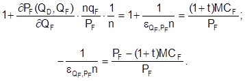
Domestic firm maximizes its profit given the price set in the foreign car market. F. O. C. for profit maximization are as follows:
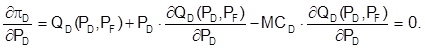
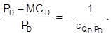
After a simple algebraic transformation F. O. C. is transformed into:
I’ll further assume that the impact of the choice
variables on relevant elasticities is as follows:  and
and
 (that corresponds to the increasing
elasticity of demand when the price of the other goods decreases). The market
equilibrium is found as an interaction of the two optimality conditions, and
can be visualized with the help of a graph (figure). The rD and rF
lines represent the optimal response functions of domestic and foreign sectors,
respectively. Applying Nash equilibrium concept, the markets will equilibrate
at prices PD* and PF* for domestic
and foreign cars.
(that corresponds to the increasing
elasticity of demand when the price of the other goods decreases). The market
equilibrium is found as an interaction of the two optimality conditions, and
can be visualized with the help of a graph (figure). The rD and rF
lines represent the optimal response functions of domestic and foreign sectors,
respectively. Applying Nash equilibrium concept, the markets will equilibrate
at prices PD* and PF* for domestic
and foreign cars.
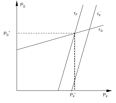
Figure. The graph of the market equilibrium
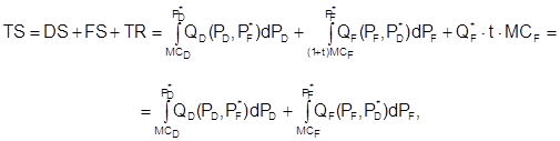
Stage 1. At this stage government decides how to set a tariff to maximize the total surplus in the automobile market. For this calculation government ignores the question of distributing the surplus among consumers and producers. Thus, the total surplus is calculated as follows:
Уважаемый посетитель!
Чтобы распечатать файл, скачайте его (в формате Word).
Ссылка на скачивание - внизу страницы.