Вища математика: Навчальний посібник (англійською мовою), страница 2

- the column vector of the right-hand side of the system

 

- the column vector of the unknowns

Let’s pass to the next method called Cramer’s rule. It shows explicitly ясно how the solutions depend on the elements of the augmented matrix.

Theorem (Cramer’s rule). The system (1) has a unique solution if Δ≠0, namely

 

where

(Δ_i – the determinant of the matrix formed by replacing the i-th column of the coefficient matrix A by the column vector B of the right-hand side of the system)

So, to use Cramer’s rule we should check the following two conditions: 1) the linear system is square; 2) its Δ≠0.

Example.

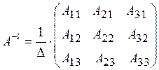
6. Let’s recall the definition of the inverse matrix A^-1:

It is a matrix which satisfies the following condition:

 

The inverse matrix can be found by the formula:

 

Let’s return to the linear system (1) and consider it in the matrix form:

 

=

Consider the same in short form:

.

Multiplying the both sides of this equation by A^-1 we get:

,    

According the definition of the inverse matrix (I mean                        ) we get the formula:

 

(2)

So, if Δ≠0 for the system (1), then it has a unique solution, which can be found by the formula (2) (matrix method).

Topic “Gauss Methodand Gauss-Jordan Method”

1. Themaindefinitions.

2.Gauss Method.

3.Implementation of the Gauss method in different cases.

4.Gauss-Jordan Method.

1. Definition. A linear equation in variables x₁, x₂, ..., x_n has the form

,            (1)

where the numbers a₁, a₂, ..., a_n are the equation’s coefficients and b is a coefficient of the right-hand side of the equation.

What can we say about the solution of the given equation? (For your example?) Really, the fixed values of variables x, y, z will be a solution of this equation, if substituting these values for the variables into the equation gives a true statement. So we have the following definition:

Definition. The ordered sequence of n numbers (s₁, s₂, ..., s_n) is the solution of the equation (1), if it satisfies this equation.

Remark. The ordered sequence of n numbers is often called n-tuple.

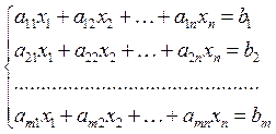
Now consider a system of linear equations. In common case it has the form:

 

(2)

Definition. The system of linear equations (2) has the solution (s₁, s₂, ..., s_n), if this n-tuple is a solution of all of the equations in the system.

To solve the system means to find the set of all solutions.

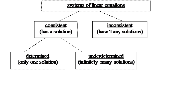
The system is called a consistent one if it has some solutions. It is called an inconsistent one if it has no solutions.

What do you think about the number of solutions of the linear system?

To discuss this problem let’s consider the system with two equations and two variables:

In this case each equation describes the straight line in the plane. So we should study the mutual location of these lines. There are three cases: the lines intersect (therefore we have one solution), the lines are parallel(there are no solutions) and the lines coincide (there are infinitely many solutions). There is the same situation in common case:

2. Let’s pass to the methods of solution of the systems of linear equations. One of the important methods is Gauss Method which also called Gaussian Elimination. It transforms the system, step by step, into one with a form that is easily solved.

The next example introduces this algorithm.

So, let’s consider a typical use of Gauss method.

Example 1.

(The “empty place” means that the coefficient of z equals zero, so the corresponding term is absent)

Let’s begin to reduce the system by sequential eliminations.

The first transformation of the system involves using the first equation to eliminate the x in the second and third equations. To get rid of the 2x in the second equation we multiply the both sides of the first equation by (-2), add that to the corresponding sides of the second equation and write the result in as a new second equation. To get rid of the x in the third equation we multiply the both sides of the first equation by (-1), add that to the corresponding sides of the third equation and write the result in as a new third equation. By the way the first equation is called the pivot equation (ведущий, розв’язувальний) and the x is called the leading variable. After these transformations we have got the following system: