Вища математика: Навчальний посібник (англійською мовою), страница 15

1) find the critical points of function within the region D (according to point 1 of the lecture outlook);

2) calculate the values of function at these points;

3) find the greatest and smallest function values of the region boundary (according to point 2);

4) compare these values and set a global maximum and a global minimum.

Let’s consider the condition of the following problem:

Find the greatest and smallest values of the function                    in the region

 

I suggest you work at this problem on your own.

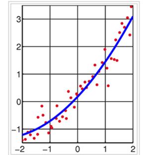
4. I’d like to startwith so-called curve fitting. Curve fitting is the process of constructing a curve, or mathematical function, which has the best fit to a series of data points:

(For example we have the set of red points and we should find the curve, which has the best fit to these points. Mark thesepointson thechart. In this situation the curve was obtained in assumption that it’s defined by the quadratic function)

The result of fitting a set of data points with a quadratic function.

The Least Squares method (abbreviated - LSM) solves these problems.

Let’s consider some practical problems which can be solved with the help of this method.

1)  The dependence between the advertising costs (x) and sales (y):

2)  The dependence between the oil price (x) and oil shares (y):

(We have some tendency and we want to forecast the next value - in assumptionthat tendency has continued. Or we can want to forecast the approximate value of index y which corresponds to the missing value of factor x)

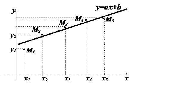
One of the important special cases of this problem is finding the straight line (and its equation) which fits best to the given points (i.e. line passesbetweenthe points). So we need to find the equation of this line, which has the form y=ax+b, more exactly, we need to find its coefficients  a  and  b.

We will deal with the linear case only. The corresponding figure is lower.

 

Really we have 5 points with their coordinates and we are looking for the line located between these points as close as possible to all points. We must do it the best way in a certain sense, namely, the best fit in the least-squares sense minimizes the sum of squared residuals, a residual being the difference between an observed value and the fitted value provided by a model.

In more common case we have the data set which consists of n points (x_i; y_i), i=1, …, n, where x_i is an independent variable and y_i is a dependent variable whose values are found by observation:

The model function has the form  y=ax+b. The goal is to find the parameter values for the model which "best" fits the data. The least squares method finds its optimum when the sum S of squared residuals is a minimum.

Thus we calculate the squared residuals, find their sum (add up them) and try to minimize this value. As a result we have the problem of extremum of function of two variables.

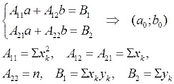
We omit the process of solving of this task and we will use only the result. The result is a system of linear equations for finding the coefficients a and b of the equation  y=ax+b.

Let’s сonsider another example:

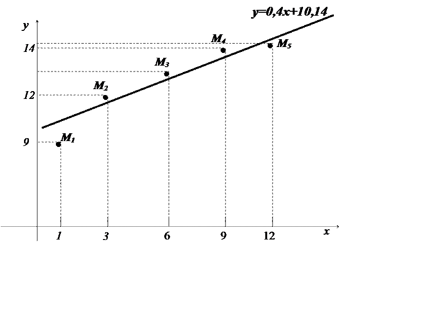
Example. Investigate the dependence of profitability of some shares from time using the observational data:

According to the LSM- method we should create the system: