We can see that this system coincides with the prior one with the exception of the last coefficient. So we can begin similarly:
 |
After these eliminations we got two identity equations, therefore we have redundant equation. So we can throw away the last equation. Now we have the system with more variables than equations:
 |
We can see that if we assign any fixed value for z we will get the proper value of y (from the second equation); after that we can find the proper value of x. If we change the value of z we will get other values of y and x. So we have got the infinite number of solutions. In this case the unknown z is called a free variable.
So let’s denote z=C, where C
is an arbitrary constant. From the second equation we get the
expression for y:  , after that
from the first equation we get the expression for x (substituting
corresponding expressions for z and y):
 .
.
Thus, we can see that the solution set contains the infinite number of elements and it can be described as

 , z=C, where C is an
arbitrary constant.
For instance, taking z=0 gives  and
and  .
.
I would like to notice that a linear system can have more than one variable free.
Example 5.
х1 + х2 +х3 - х4 = 1
х2 - х3 + х4 = -1
3х1 + 6х3 -6х4 = 6
-х2 +х3 - х4 = 1
The elementary operations give us the following equivalent system:
х1 + х2 +х3 - х4 = 1
х2 - х3 + х4 = -1
0 = 0
0 = 0
To get the solution we will start at the bottom. We first express x2 in terms of the free variables x3 and x4, putting x3=C1, x4=C2:
х2 =C1- C2 -1.
Next, moving up to the first equation substitute for х2:
х1 + C1- C2 -1 + C1– C2 = 1
Solving for x1 yields:
x1 = 2 - 2C1 + 2C2 , where C1, C2 are arbitrary constants.
So we got an answer: x1 = 2 - 2C1 + 2C2 , х2 =C1- C2 -1, where C1, C2 are arbitrary constants.
I’d like to draw your attention that we considered the so-called square systems (which have the same numbers of equations as unknowns), but we can apply this method to solve any linear system (for any size and in case of non-coincidence of the numbers of equations and unknowns). In this sense Gauss method is universal).
Example 6.
х1 + 2 х2 = 1
2х1+ х3 = 2
3х1 +2х2 + х3 -х4 = 4
Topic “The general theory of the linear systems”
1. The definition of the rank of a matrix.
2. The computing of the rank of a matrix.
3. Investigation of the linear system for consistency.
4. Homogeneous linear system.
 |
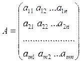
1. - n by m matrix
Delete any k rows and any k columns. The deleted elements create k-order determinant. It is called the k-order minor of the matrix A.
Definition. The rank of a matrix is the greatest order of any non-zero minor of the matrix.
 ,
,  ,
rank - ?
2. The definition does not give an efficient way of computing of the rank.
So, we need the ways of calculations of the matrix rank.
The method which we are going to use is the computing of the rank from row-echelon form, which we can get with the help of the elementary row operations, such as follows:
1) interchanging two rows;
2) multiplying a row by a non-zero scalar;
3) adding a multiple of one row to another row;
4) deleting a zero-row or a repeating row.
Remark. Elementary row operations do not change the rank of a matrix.
A common approach to finding the rank of a matrix is to reduce it to the row-echelon form (to the triangle form). The rank will be equal to the maximum possible number of non-zero elements of the main diagonal.
Examples:
 |
 |
;
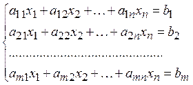
3. A system of m linear equations with n unknowns can be written as
 |
||
 |
||
- the coefficient matrix,
 |
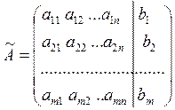
- - the augmented matrix,
Уважаемый посетитель!
Чтобы распечатать файл, скачайте его (в формате Word).
Ссылка на скачивание - внизу страницы.