One of the principal input parameters to the model is the inter-particle interaction potential. In the current study, the inter-particle potential is modeled by DLVO theory [22,23]:
VTOT = VVDW + VEDL (8)
where VVDW is the van der Waals’ potential and VEDL the electrostatic double layer potential. The attractive van der Waals’ potential between equal-sized particles can be modeled by many available expressions. In this study, it is calculated by [24]:
![]() (9)
(9)
where AH is the Hamaker constant and s=r/a the dimensionless center-to-center separation between two particles scaled
by the particle radius a.
The electrostatic interaction potential between the particlesiscalculatedfromthelinearsuperpositionapproximation of Bell et al. [25] and Chew and Sen [26]:
VEDL = ![]() (10)
(10)
![]() (11)
(11)
κ−1 =(12)
 AI
AI
where κ−1 is the Debye screening length, NA the Avogadro’s number, I the ionic strength of the solution, εr the dimensionless dielectric permittivity of water, ε0 the permittivity of free space, n0 the ion number concentration, kB the Boltzmann’s constant, T the absolute temperature, zs the valence of ions in the bulk solution, e the charge of an electron, and ψs the surface potential of the particles which can be substituted by the zeta potential [27].
The second primary physical parameter inputted into the current model is the hydrodynamic drag. The expression for the hydrodynamic drag force derives directly from Stoke’s law for a single particle in an infinitely unbounded medium:
FStokes = 6πµav (13)
where µ is the fluid viscosity and v the permeate velocity. For fluid flow through a porous medium composed of equal-sized spherical particles, the true hydrodynamic drag force exerted on each particle within the medium is adjusted by Happel’s correction factor Ω, defined earlier in Eq. (7), [19]:
Fhydro = FStokesΩ (14)
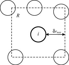
Fig. 2. Range of particle displacements for Monte Carlo simulation.
Monte Carlo simulation (MC) is a stochastic modeling method that is especially suitable to problems involving the dynamics of particle motion because of its capability to evaluate each discrete particle displacement. A classical method for performing MC begins by casting the process as being Markovian, meaning that the outcome for a particle displacement depends solely on the outcome that immediately precedes it. The system progresses from one state to the next by aid of its transition probability matrix. Metropolis et al. [28] present the now standard Metropolis method for conducting MC simulations using the energy of the system as the criterion to evaluate the acceptance or rejection of a MC step.
The Metropolis method begins by considering a system of particles as shown in Fig. 2. The particle of interest i is initially located at rim. Particle i is then proposed to be displaced randomly to a new location rin using the algorithm:
rin = rim + (2a0 − 1)δrmax (15)
where a0 is a uniform random number between 0 and 1 and δrmax the maximum allowable displacement. The proposed displacement is next evaluated for acceptance or rejection. The criterion for acceptance is the change in potential energy Vn,m of the system computed as
 ) (16)
If Vn,m <0, then the proposed move is downhill and accepted. If Vn,m >0, the proposed move is uphill and is accepted with the qualification of the probability ρn/ρm which in the Metropolis method corresponds to the Boltzmann factor of the energy difference:
Уважаемый посетитель!
Чтобы распечатать файл, скачайте его (в формате Word).
Ссылка на скачивание - внизу страницы.