Validation for the Cox Model. Terry M. Therneau Mayo Foundation. Breslow estimates. Exact partial likelihood

Validation for the Cox Model

Terry M. Therneau Mayo Foundation

Oct 2010

It is useful to have a set of test data where the results have been worked out in detail, both to illuminate the computations and to form a test case for software programs. The data sets below are quite simple, but have proven useful in this regard.

1  Test data 1

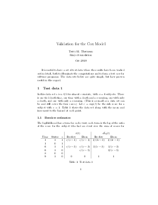
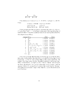
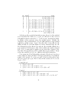
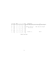
In this data set x is a 0/1 treatment covariate, with n = 6 subjects. There is one tied death time, one time with a death and a censoring, one with only a death, and one with only a censoring. (This is as small as a data set can be and still cover the four cases.) Let r = exp(β) be the risk score for a subject with x = 1. Table 1 shows the data set along with the mean and increment to the hazard at each point.

1.1  Breslow estimates

The loglikelihood has a term for each event; each term is the log of the ratio of the score for the subject who had an event over the sum of scores for

Table 1: Test data 1

those who did not.

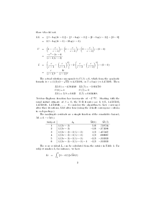
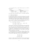
       The actual solution corresponds to√   U(β) = 0, which from the quadratic

formula is r = (1/2)(3 +         33) ≈ 4.372281, or β^ˆ = log(r) ≈ 1.475285. Then

                                   LL(0) = −4.564348      LL(β^ˆ) = −3.824750

                                   U(0) = 1                           U(β^ˆ) = 0

I(0) = 5/8 = 0.625 I(β^ˆ) = 0.634168.

Newton–Raphson iteration has increments of −I⁻¹U. Starting with the usual initial estimate of β = 0, the N–R iterates are 0, 8/5, 1.4727235, 1.4752838, 1.4752849, .... S considers the algorithm to have converged after three iterations, SAS after four (using the default convergence criteria in each package).

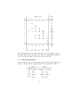
The martingale residuals are a simple function of the cumulative hazard, M_i = δ_i − rΛ(^ˆ t_i).

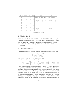
The score residual L_i can be calculated from the entries in Table 1. For subject number 3, for instance, we have

.

Let a = (r + 1)(3r + 3) and b = (r + 3)²; then the residuals are as follows.

The Schoenfeld residuals are defined at the three unique death times, and have values of 1−r/(r +1) = 1/(r +1), {1−r/(r +3)}+{0−r/(r +3)} = (3 − r)/(3 + r), and 0 at times 1, 6, and 9, respectively. For convenience in plotting and use, however, the programs return one residual for each event rather than one per unique event time. The two values returned for time 6 are 3/(r + 3) and −r/(r + 3).

The Nelson–Aalen estimate of the hazard is closely related to the Breslow approximation for ties. The baseline hazard is shown as the column Λ₀ above. The hazard estimate for a subject with covariate x_i is Λ_i(t) = exp(x_iβ)Λ₀(t) and the survival estimate is S_i(t) = exp(−Λ_i(t)).

The variance of the cumulative hazard is the sum of two terms. Term 1 is a natural extension of the Nelson–Aalen estimator to the case where there are weights. It is a running sum, with an increment at each death time of dN(t)/(^PY_i(t)r_i(t))². For a subject with covariate x_i this term is multiplied by [exp(x_iβ)]².