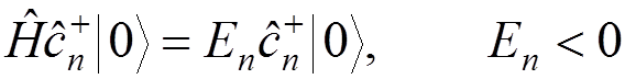
 ,
,
 are eigenvalues of
  .
.
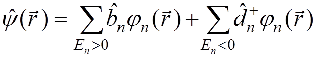
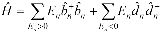
Spectrum of the Dirac equation for the Coulomb field:
![]()
![]()
positive-energy-continuum states
![]()
![]()
 ___________________________
![]() ________________________________________
________________________________________
ß bound states
_________________________________________
0 _ _ _ _ _ _ _ _ _ _ _ _ _ _ _ _ _ _
![]()
negative-energy-continuum states
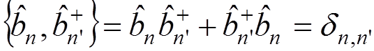
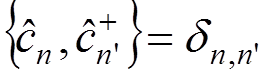
![]() and
and ![]() are the operators satisfying the following anticommutation relations
are the operators satisfying the following anticommutation relations
 ,
,
 ,
,

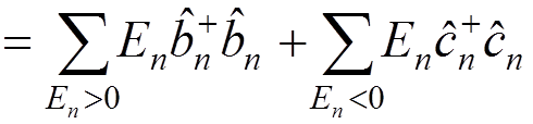
The energy operator
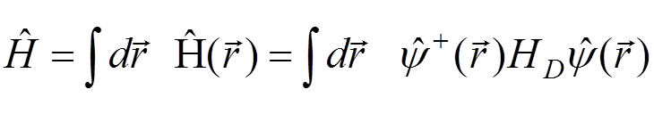
 .
.
As usual, the vacuum state is defined by
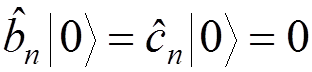 .
.
Then, we have
 ,
,
 .
.
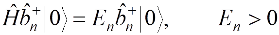
Let us consider a state
 .
.
Its energy

is not restricted from the bottom! For this reason, let us redefine the vacuum state
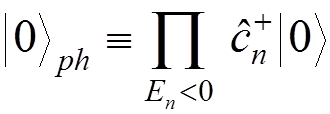 .
.
For the new vacuum, we have
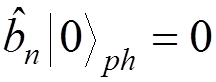 , for any
 ![]() ,
,
 , for any
 ![]() .
.
If we denote
 ,
,
we get
 , for any
 ![]() .
.
In what follows, we imply
 .
.
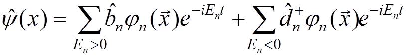
The  operator:
 .
.
The
physical sense of  and
and  :
:
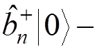
is a creation operator for
electrons,
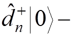
is a creation operator for
positrons.
Therefore,
 a one-electron
state,
a one-electron
state,
 a one-positron state.
The energy operator
 .
.
 .
.
The last term represents the vacuum energy. It can be removed by using the normal product:
 .
.
The electric charge density for the vacuum state:
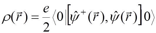
 .
.
Here  . In the free-field case
  ,
,
the
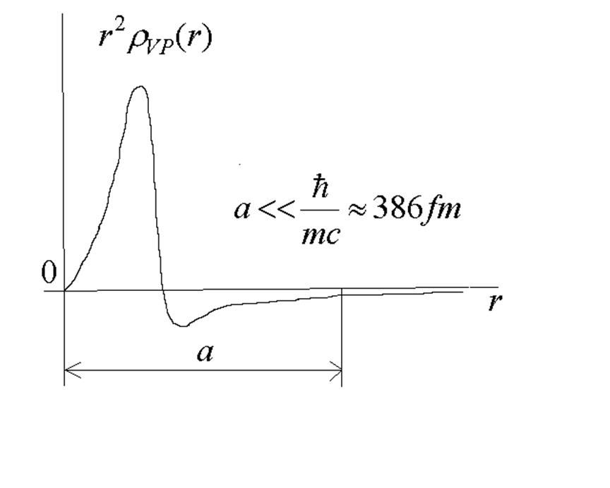
two sums cancel each other. For
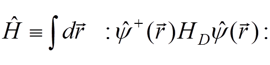
the Coulomb field of a nucleus,  , the functions
  for
for
 are pulled closer to the nucleus while for
 are pushed out. For the case of an
extended heavy nucleus, it yields the following picture for the
vacuum-polarization charge density multiplied with
are pushed out. For the case of an
extended heavy nucleus, it yields the following picture for the
vacuum-polarization charge density multiplied with ![]() (after
renormalization):
(after
renormalization):
Vacuum-polarization
charge density multiplied with ![]() for a heavy extended
nucleus :
for a heavy extended
nucleus :
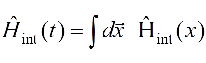
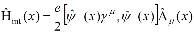
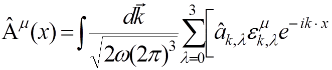
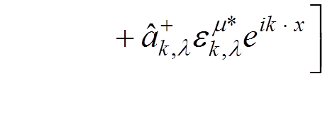
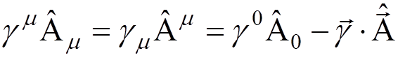
QED of interacting fields
In what follows, we will use the relativistic units:
![]() .
.
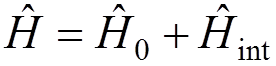
The Hamiltonian of the system:
 ,
,
where, in the Coulomb gauge,
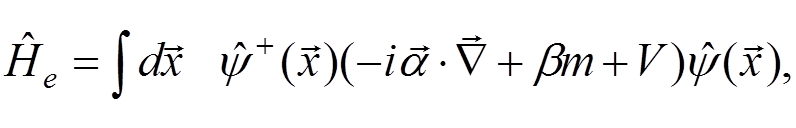
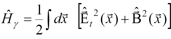 ,
,
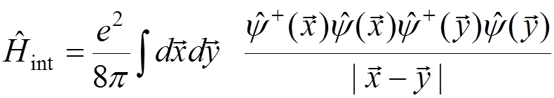
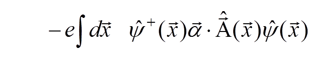 .
.
The calculations can be performed by perturbation theory.
However, manifestly covariant expressions, which are required for the renormalization , can be most readily obtained if we use the interaction representation instead of the Schroedinger or the Heisenberg representation. The Hamiltonian of the system:
 ,
,
where 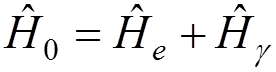 .
.
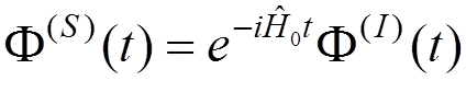
The Schroedinger representation:
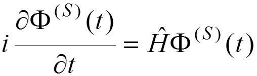 .
.
For any
operator ![]() :
:
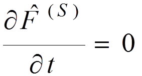 .
.
The
average value of ![]() :
:
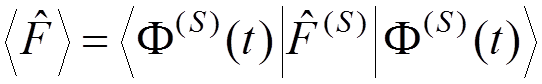 .
.
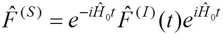
The transition to the Heisenberg representation is performed by the substitutions:
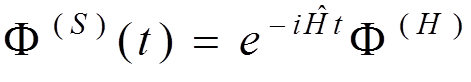 ,
,
 .
.
We have
 ,
,
 .
.
The
average value of ![]() :
:
 .
.
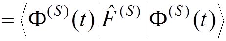
Interaction representation
 ,
,
 ,
,
we obtain
 ,
,
 .
.
The
average value of ![]() :
:
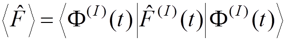
.
In what follows, we will consider the interaction representation. In the Feynman gauge
 ,
,
where
 ,
,
 ,
,
![]()
 .
.
Here  ,
,  ,
,
 ,
,  ,
,  ,
,  .
.
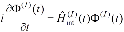
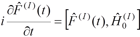
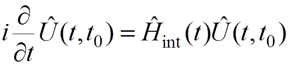
In the
interaction representation, the wave function  obeys
the equation
obeys
the equation
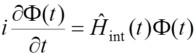 ,
,
Let us
introduce the evolution operator 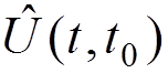 by
by
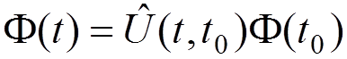 .
.
We obtain
with the boundary condition
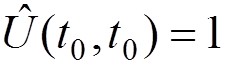 .
.
These equations can be combined into a single integral equation
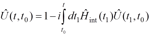 .
.
Уважаемый посетитель!
Чтобы распечатать файл, скачайте его (в формате Word).
Ссылка на скачивание - внизу страницы.