We repeated this procedure by changing the assumption that the values in Table II were valid for series with another frequency of observation (biweekly, weekly, daily or intraday). Afterwards, we considered another series, say a monthly series, and repeated the whole process anew. Finally, we studied the resulting trends with different percentages of smoothness, particularly with 65% and 85% smoothness, by visual inspection. It should be stressed that this kind of analysis was required for the ES filter and not for the HP filter because the latter arose naturally when analyzing quarterly economic time series.

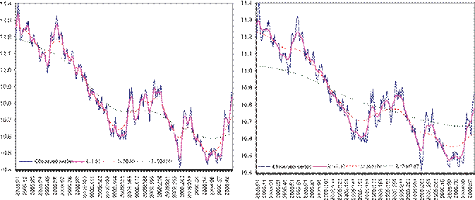
Figure 4. Daily exchange rate (Pesos/U.S. Dollar). Observed series and trends with: S%=65% (left): daily
(=1.81), weekly (=50.80) and monthly (=934.90); S%=85% (right): daily (=11.10), weekly (=305.49) and monthly (=7407.87).
In Figure 4 we present the daily Exchange Rate (Mexican Pesos/U.S. Dollar) series and two trends, with 65 and 85% smoothness respectively, for different frequencies of observation (daily, weekly and monthly). The sample period runs from January, 2005 to March, 2006. We obtained the trends for the different periodicities by assuming that the value of for each periodicity was given as in Table II and applied the results of the previous section to obtain the equivalent value of the smoothing constant for the daily series.
![]() Using a daily basis we get N =319
and =1.810. The graph in the left of
Figure 4 allows us to see that the trend neither emphasizes the fit to the data
nor its smoothness, which is what we expect to see for 65% of smoothness. Now,
in the weekly case with N =63
we get =1.872 from Table II, then we
assume 5-day weeks (i.e. n=20,
k=5 and
Using a daily basis we get N =319
and =1.810. The graph in the left of
Figure 4 allows us to see that the trend neither emphasizes the fit to the data
nor its smoothness, which is what we expect to see for 65% of smoothness. Now,
in the weekly case with N =63
we get =1.872 from Table II, then we
assume 5-day weeks (i.e. n=20,
k=5 and ![]() 872) to obtain =50.80 from expression (32). In this case, the figure
shows an apparent undue emphasis of smoothness over fit of the trend. This fact
is even more pronounced in the monthly case, where we used N =15, n=5, k 171 and =934.90. Moreover, we could not assume a quarterly
series because we would have N =1
and the method requires at least three quarters to produce a trend with 65%
smoothness. The graph in the right of Figure 4 shows results similar to those
of the previous exercise, but now with 85% smoothness. Using a daily basis we
have N
872) to obtain =50.80 from expression (32). In this case, the figure
shows an apparent undue emphasis of smoothness over fit of the trend. This fact
is even more pronounced in the monthly case, where we used N =15, n=5, k 171 and =934.90. Moreover, we could not assume a quarterly
series because we would have N =1
and the method requires at least three quarters to produce a trend with 65%
smoothness. The graph in the right of Figure 4 shows results similar to those
of the previous exercise, but now with 85% smoothness. Using a daily basis we
have N ![]() 104 and the
resulting trend shows a smooth long-term behavior, while keeping a reasonable
fit to the data. With
104 and the
resulting trend shows a smooth long-term behavior, while keeping a reasonable
fit to the data. With
![]()
![]() weekly (N 5 and =305.486) and monthly (N
weekly (N 5 and =305.486) and monthly (N
and =7407.871) bases the trend overemphasizes smoothness and tends to behave as a constant mean.
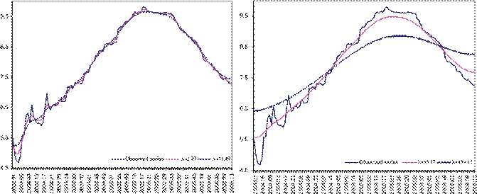
The following exercise considers the weekly yield rate of the Mexican federal funds called CETES28. This series is shown in Figure 5 together with its trend with 85% of smoothness. Since

![]() Figure 5. Weekly yield
rate of CETES28 and its trend with 85% smoothness. Left: dailyand weekly (=11.49). Right: monthly (=55.17) and quarterly
Figure 5. Weekly yield
rate of CETES28 and its trend with 85% smoothness. Left: dailyand weekly (=11.49). Right: monthly (=55.17) and quarterly ![]() .
.
the sample covers data from January, 2004 to March, 2006 (n=117 weeks) the trend for daily
data is obtained by assuming N =585
days, so that ∗5=11.007. The series is of stocks, thus for the weekly
case we get from expression (32) k![]() 2.201. Now, by considering the
weekly data directly we know that N =117,
thus we get
2.201. Now, by considering the
weekly data directly we know that N =117,
thus we get ![]() 491 from Table II.
491 from Table II.
In the right of that figure we also show
the corresponding exercise with monthly and quarterly periodicity. For the
monthly data we assumed N =29,
so that =13.792. As a result, for monthly
data we have k=4
and ![]() 168. For quarterly data
(with N =9
quarters) we obtained = 33.780, consequently we used k=13 to produce
168. For quarterly data
(with N =9
quarters) we obtained = 33.780, consequently we used k=13 to produce ![]() 133. It should be noticed
that as the basis period increases, the trend becomes smoother. When the
periodicity is daily or weekly, the trend shows a balance between smoothness
and fit. On the other hand, if a monthly or quarterly basis is used, the
smoothness component is over-emphasized. Thus, in this example neither the
monthly nor the quarterly periodicities seem suitable as the standard basis of
reference for trend smoothness.
133. It should be noticed
that as the basis period increases, the trend becomes smoother. When the
periodicity is daily or weekly, the trend shows a balance between smoothness
and fit. On the other hand, if a monthly or quarterly basis is used, the
smoothness component is over-emphasized. Thus, in this example neither the
monthly nor the quarterly periodicities seem suitable as the standard basis of
reference for trend smoothness.
Уважаемый посетитель!
Чтобы распечатать файл, скачайте его (в формате Word).
Ссылка на скачивание - внизу страницы.