МІНІСТЕРСТВО ОСВІТИ І НАУКИ УКРАЇНИ
НТУ «ХПІ»
Кафедра обчислювальної техніки та програмування
ЗВІТ З ЛАБОРАТОРНОЇ РОБОТИ № 2
З КУРСУ: «ПЛАНУВАННЯ ЕКСПЕРИМЕНТУ ТА ОБРОБКА ЕКСПЕРИМЕНТАЛЬНИХ ДАНИХ»
Виконав студент
гр. КІТ -14в
Марченко В.Ю.
Перевірив:
Черних О.П.
Харків 2006
Лабораторна робота №2
Тема: Перевірка статичних даних.
Мета роботи: перевірка статистичних гіпотез для однієї та двох вибірок.
Порядок виконання роботи:
За допомогою програми StatWizard створюємо дані що містять 3 вибірки, сформовані з випадкових цілих чисел у діапазоні 1-30. Розміри виборок – 50,75 та 100.
1.
1 3 5 4 2 12 30 29 7 13 17 6 9 19 8 5 4 3 23 27 29 20 11 15 1 3 5 4 2 3 3 8 7 16 17 17 12 11 3 13 30 12 10 9 7 8 6 4 2 2
2.
2 22 13 15 26 5 30 9 7 6 8 7 13 12 14 11 16 19 20 3 16 13 12 15 4 3 1 3 3 3 2 5 4 8 10 10 11 16 17 24 21 24 26 28 24 2 13 16 15 19 10 1 2 7 5 17 23 21 20 30 14 12 15 10 9 6 3 2 2 6 1 15 16 19 1
3.
2 4 13 12 11 15 20 21 30 1 4 4 3 5 7 6 8 16 17 18 13 12 14 4 5 9 7 10 10 2 5 4 13 12 12 16 4 30 29 25 29 1 2 14 15 2 6 8 7 4 2 13 15 1 11 17 22 22 24 26 25 21 20 15 16 4 3 18 6 9 11 14 10 1 17 4 2 8 10 6 16 14 5 18 14 12 10 26 21 22 28 30 1 12 16 17 12 10 2 7
Вибірка№1
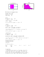
1) Переходимо в процедурний блок “Describe_Numeric Data-One-Variable_Analysis”,
проводимо розрахунок статистичних даних для першої вибірки і порівнюємо їх з самостійно виконаними розрахунками
Робимо аналітичний розрахунок заданих статистичних характеристик.
Мат. Очікування:
 = 10.3400
a=[1 3 5 4 2 12 30 29 7 13 17 6 9 19 8 5 4 3 23 27 29 20 11 15 1 3 5 4 2 3 3 8 7 16 17 17 12 11 3 13 30 12 10 9 7 8 6 4 2 2]
>> sum(a)
ans =
517
>> M=ans/50
M =
10.3400
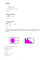
Дисперсія:
 =69.3718
>> a1=(a-M).^2
a1 =
Columns 1 through 11
87.2356 53.8756 28.5156 40.1956 69.5556 2.7556 386.5156 348.1956 11.1556 7.0756 44.3556
Columns 12 through 22
18.8356 1.7956 74.9956 5.4756 28.5156 40.1956 53.8756 160.2756 277.5556 348.1956 93.3156
Columns 23 through 33
0.4356 21.7156 87.2356 53.8756 28.5156 40.1956 69.5556 53.8756 53.8756 5.4756 11.1556
Columns 34 through 44
32.0356 44.3556 44.3556 2.7556 0.4356 53.8756 7.0756 386.5156 2.7556 0.1156 1.7956
Columns 45 through 50
11.1556 5.4756 18.8356 40.1956 69.5556 69.5556
>> D=(sum(a1))/49
D =
69.3718
Стандартне відхилення:
![]() =8.3290
=8.3290
>> otk=sqrt(D)
otk =
8.3290
Стандартна помилка:
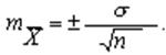 = 1.1779
>> osh=otk/sqrt(50)
osh =
1.1779
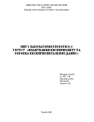
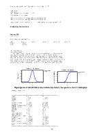
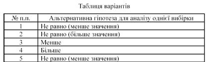
2) Згідно індивідуального завдання перевіряїємо гіпотезу для аналізу однієї вибірки відносно оцінки мат. очікування (варіант№ ) та виконуємо побудову гістограм та графіків „Box and Whisker”
Виконаємо дії по перевірці гіпотез.
Hypothesis Tests for X1
Sample mean = 10,34
Sample median = 8,0
t-test
------
Null hypothesis: mean = 10,34
Alternative: less than
Computed t statistic = 0,0
P-Value = 0,5
Do not reject the null hypothesis for alpha = 0,05.
sign test
---------
Null hypothesis: median = 10,34
Alternative: less than
Number of values below hypothesized median: 30
Number of values above hypothesized median: 20
Large sample test statistic = 1,27279 (continuity correction applied)
P-Value = 0,101546
Do not reject the null hypothesis for alpha = 0,05.
signed rank test
----------------
Null hypothesis: median = 10,34
Alternative: less than
Average rank of values below hypothesized median: 24,1667
Average rank of values above hypothesized median: 27,5
Large sample test statistic = 0,840237 (continuity correction applied)
P-Value = 0,200387
Do not reject the null hypothesis for alpha = 0,05.
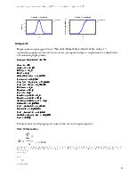
Probability Distributions
Inverse CDF
-----------
Distribution: Student's t
CDF Dist. 1 Dist. 2 Dist. 3 Dist. 4 Dist. 5
0,975 2,00958
0,95 1,67655
The StatAdvisor
---------------
This pane finds critical values for the Student's t distribution.
You may specify up to 5 five tail areas. The critical value is
defined as the largest value for the Student's t distribution such
that the probability of not exceeding that value does not exceed the
area specified. For example, the output indicates that, for the first
distribution specified, 2,00958 is the largest value such that the
probability of not exceeding 2,00958 is less than or equal to 0,975.
Уважаемый посетитель!
Чтобы распечатать файл, скачайте его (в формате Word).
Ссылка на скачивание - внизу страницы.