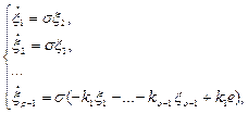
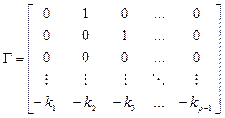
define the purpose of control as the solution of the problem of synthesizing the algorithm which at any initial conditions ensures the boundedness of all system signals as well as the execution of purpose condition
![]() , (3)
, (3)
for some ![]() , where
, where ![]() is a tracking error,
is a tracking error, ![]() – a number which can be decreased by control law
selection.
– a number which can be decreased by control law
selection.
3. CONTROL DESIGN
We rewrite the system (1) in the following form
 (4)
(4)
where ![]() ,
, ![]() , …,
, …, ![]() -
- ![]() vectors;
vectors; ![]() ,
, ![]() , …,
, …, ![]() –components of the vector of unknown time-varying parameters
–components of the vector of unknown time-varying parameters ![]() .
.
The state-space model (4) can be represented in the input-output form
![]() (5)
(5)
where ![]() – differentiation operator, transfer function
– differentiation operator, transfer function ![]() .
.
Before beginning the synthesis of control law let us formulate the auxiliary result published in [14]. Consider linear system time-invariant system
![]() (6)
(6)
where ![]() ,
, ![]() ,
, ![]() . Transfer function of system (6) is
determined by expression
. Transfer function of system (6) is
determined by expression ![]() .
.
Let the system (6) be closed
![]() , (7)
, (7)
in which number ![]() .
.
Let us put a question about
existence of positively defined matrix ![]() and number
and number ![]() satisfying the correlations
satisfying the correlations
![]() , (8)
, (8)
![]() (9)
(9)
for some positively defined
matrix ![]() .
.
Lemma [14],[15]. Let ![]() , where
, where ![]() and
and ![]() . Let
. Let ![]() be a Hurwitz polynomial and
be a Hurwitz polynomial and ![]() then exists a number
then exists a number ![]() for which correlations (8), (9) are
solvable for any
for which correlations (8), (9) are
solvable for any![]() .
.
Choose the control law of the following form
![]() , (10)
, (10)
where ![]() is a positive number; the positive parameter
is a positive number; the positive parameter ![]() is intended for compensation of the uncertainties
is intended for compensation of the uncertainties ![]() and
and ![]() ; polynomial
; polynomial ![]() is chosen for the polynomial
is chosen for the polynomial ![]() to be Hurwitz and (
to be Hurwitz and (![]() ) order; function
) order; function ![]() is the estimate of signal
is the estimate of signal ![]() which is calculated according to the following algorithm
which is calculated according to the following algorithm
 (11)
(11)
![]() , (12)
, (12)
where number ![]() ( calculation procedure of
( calculation procedure of ![]() is presented in Appendix, inequality (A.8)), and parameters
is presented in Appendix, inequality (A.8)), and parameters ![]() are calculated for the system (11) to be
asymptotically stable for input
are calculated for the system (11) to be
asymptotically stable for input ![]() .
.
Substituting (10) in equation
![]() we obtain
we obtain
![]()
![]()
![]() (13)
(13)
where deviation function ![]() equals
equals
![]() . (14)
. (14)
Transform the equation (13) in the following way
![]()
Let us introduce the
following indication ![]() ,
,
where according to the
polynomial ![]() is Hurwitz, parameters
is Hurwitz, parameters ![]() are bounded and smooth, signal
are bounded and smooth, signal ![]() and its derivatives up to order
and its derivatives up to order ![]() including we obtain
including we obtain ![]() is bounded.
is bounded.
Then for equation (13) obtain
![]()
![]() .
.
Let us denote ![]() ,
, ![]() ,
,
then for (13) we have
![]() , (15)
, (15)
where according to the
polynomial ![]() is Hurwitz and function
is Hurwitz and function ![]() is bounded we obtain
is bounded we obtain ![]() is also bounded.
is also bounded.
Rewrite the input-output model (15) in state-space form
 (16)
(16)
As ![]() is (
is (![]() ) order Hurwitz polynomial then in view of
lemma presented above number
) order Hurwitz polynomial then in view of
lemma presented above number ![]() exists that it is possible to find number
exists that it is possible to find number ![]() and symmetrical positively defined matrix
and symmetrical positively defined matrix ![]() satisfying following matrix equations
satisfying following matrix equations
![]() ,
, ![]() , (17)
, (17)
where ![]() is positively defined matrix.
is positively defined matrix.
Notice matrix ![]() parameters depend on parameter
parameters depend on parameter ![]() and do not depend on
and do not depend on ![]() .
.
Let us rewrite model (11), (12) in vector-matrix form
 (18)
(18)
where  ,
,  and
and  .
.
Consider new variable
![]() , (19)
, (19)
then according the matrix![]() structure, error
structure, error ![]() will
become
will
become ![]() .
.
For derivative of ![]() we obtain
we obtain
![]()
![]() . (20)
. (20)
As ![]() (can be checked by substitution) then
(can be checked by substitution) then
 (21)
(21)
where matrix ![]() according the calculation of parameters
according the calculation of parameters ![]() of model (11) has proper numbers with negative real
component and satisfies the Lyapunov equation:
of model (11) has proper numbers with negative real
component and satisfies the Lyapunov equation:
![]() , (22)
, (22)
where ![]() and
and ![]() are positively defined matrixes.
are positively defined matrixes.
Theorem. There exist numbers ![]() and
and ![]() such that all trajectories of system (16), (21) are bounded
and control purpose (3) is executed.
such that all trajectories of system (16), (21) are bounded
and control purpose (3) is executed.
The proof of the theorem is presented in Appendix.
4. ADAPTIVE TUNING OF PARAMETERS
In this part we consider the problem of
choosing the controller (10) – (12) parameters ![]() satisfying the theorem conditions (see expressions (A.4), (A.7) and
(A.8)). Possible variant of tuning the coefficients
satisfying the theorem conditions (see expressions (A.4), (A.7) and
(A.8)). Possible variant of tuning the coefficients ![]() is to increase them as long as the purpose condition
(3) is executed.
is to increase them as long as the purpose condition
(3) is executed.
For realization of this idea we use the following algorithm
 , (23)
where ![]() and function
and function ![]() is calculated in the following way
is calculated in the following way
 where number
 ![]() .
.
Choose ![]() in the following way
in the following way
![]() , (24)
, (24)
where number ![]() .
.
It is obvious that with such calculation of
![]() exists a point of time
exists a point of time ![]() for which, condition (17) and inequalities (A.4),
(A.7), (A.8) are executed. It is also evident that tracking error
for which, condition (17) and inequalities (A.4),
(A.7), (A.8) are executed. It is also evident that tracking error ![]() will be decreased with the rise of parameter
will be decreased with the rise of parameter ![]() (see inequality (A.12)).
(see inequality (A.12)).
5. EXAMPLE
Let us consider the following time-varying plant
 (25)
(25)
![]() , (26)
, (26)
where![]() is a measured variable;
is a measured variable; ![]() and
and ![]() – unknown variable parameters; in contrast
to work [3] we suppose that disturbance affects on the plant, i.e.
– unknown variable parameters; in contrast
to work [3] we suppose that disturbance affects on the plant, i.e. ![]() .
.
Choose control law according to equations (10) – (12)
![]() (27)
(27)
![]() , (28)
, (28)
where polynomial ![]() and coefficient
and coefficient ![]() .
.
To tune the parameters ![]() and
and ![]() we use the method proposed in the previous part. Assigning the
precision
we use the method proposed in the previous part. Assigning the
precision ![]() and command signal
and command signal ![]() we simulate the system for
we simulate the system for ![]() and
and ![]() . Results of computer simulation for unknown time-varying parameters
. Results of computer simulation for unknown time-varying parameters ![]() ,
, ![]() (given parameter values are taken from article [3]) and disturbances
(given parameter values are taken from article [3]) and disturbances ![]() on variables
on variables ![]() and
and ![]() are presented in the Fig. 1 and 2 accordingly.
are presented in the Fig. 1 and 2 accordingly.
Computer simulation graphics for ![]() and
and ![]() illustrate the achievement of proposed control purpose. It is
necessary to note that assigned adaptive control algorithm
illustrate the achievement of proposed control purpose. It is
necessary to note that assigned adaptive control algorithm
Уважаемый посетитель!
Чтобы распечатать файл, скачайте его (в формате Word).
Ссылка на скачивание - внизу страницы.