Applied stochastic models in business and industry. Trend estimation of financial time series, страница 8

where an upper bar denotes the corresponding polynomial with B replaced by B−¹ (i.e. ∇¯ k = 1−B−^k).

The values  and ∗² that make the results of both ES filters become equivalent are obtained by equating ∗₀ and ∗₁ to ₀ and _1k. That is, by asking the following system of equations to hold true:

                                                ,k       a

(29)

                                                ,k      a

where a_11,k and a_21,k are the coefficients of B⁰ and B^k in the polynomial S for a flow series or in the polynomial S_k^S¯k for a stock series. In the same way, a_12,k and a_22,k are the coefficients of B⁰ and B^k in the polynomial S_k∇k^S¯k∇¯ k for a flow series or in the polynomial ∇k∇¯ k if the series is of stocks. This system has a unique solution for ∗² and ∗², or for ² and , depending on which pair of variances is known. If the pair ∗² and ∗² is known, so that ∗_k =∗²/∗² is known, we solve the system to get

                             and                   (30)

from which it follows that  is given by

                                     −a21,k −(a11,k +2a21,^k)^∗                                                 ₍₃₁₎

Now, since ∇k∇¯ k =2−(B^k +B−^k), S_k∇kS¯k∇¯ k =2k−k(B^k +B−^k)+P_1,k(B, B−¹), S_kS¯k =k

+P_2,k(B, B−¹) and SP_3,k(B, B−¹), where P_1,k

(B, B−¹), P_2,k(B, B−¹) and P_3,k(B, B−¹) are polynomials in B and B−¹ that have no powers of type B^ik, for i =0,1. By inspection of the polynomials involved, we found for flows a_11,k =(2k³+k)/3, a_21,k =(k³−k)/6, a_12,k =2k and a_22,k =−k, whereas for stocks, a_11,k =k, a_21,k =0, a_12,k =2 and a_22,k =−1. Therefore, we finally get

                                                          =(k²−1)/6+k²∗_k             for flows

(32) k∗_k                for stocks

When the smoothing constant for the disaggregated series is known, it should be clear that we can also use expression (32) to solve for the corresponding value of ∗_k.

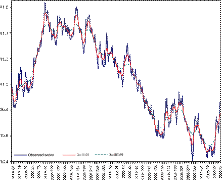
To see how the previous result works with an observed time series, let us consider the Daily Exchange Rate (Pesos/U.S. Dollar) series shown in Figure 2 together with its trend. The sample period covers data from January, 2004 to March, 2006 and considers 5-day weeks, thus the sample consists of N =580 daily observations. Table II indicates using =11.008 and =103.694 for 85% and 95% smoothness, respectively. As the percentage of smoothness grows, the trend emphasizes the smoothness component and reveals the long-term component of the series, which is what we want to see.

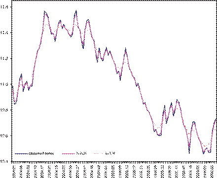
In Figure 3 we show the weekly Exchange Rate (Pesos/U.S. Dollar) series and its trend for the same period considered before. We should stress that this is a series of flows (it is the average rate for the period under consideration). The sample now consists of n=116 weekly observations, considering 5-day weeks. The values of are obtained with the formula . Therefore, the smoothing constants for the weekly series are 280 for S% 85% and 988 for S%=95%. By comparing the resulting trends with those in Figure 2, we see that trends with the same percentage of smoothness show essentially the same dynamic behavior, no matter what the frequency of observation of the data is.

Figure 2. Daily exchange rate (Pesos/U.S. Dollar) and trends with S%=85% (=11.01) and S%=95% (=103.69).

Figure 3. Weekly exchange rate (Pesos/U.S. Dollar) and trends with S%=85% (=0.28) and 95% (=3.99).

4. WHY USE DAILY DATA AS THE STANDARD FREQUENCY?

In this section we argue that the values in Table II, as well as the values obtained from the fitting models in Table III, are best suited for time series of daily observations. This argument relies on the fact that, for a given standard frequency of observation, the smoothness achieved must reflect what is expected from a trend with a given percentage of smoothness. That is, if the selected S% is high the resulting trend should emphasize smoothness over fit; while low values of S% should work in the opposite direction. Thus, we present here a few numerical examples that lend empirical support to the use of a daily series over series with other frequencies. In fact, we carried out several other analyses before reaching our conclusion of using a daily frequency of observation as standard of reference. That is, we assumed first that the value produced by the fitting model of Table II was valid for a given series, say a quarterly series, and produced the trend with such a value. Next, on the assumption that the values in Table II were valid for a monthly series and using the results in the previous section, we derived the equivalent smoothing constant for the corresponding quarterly series and produced another trend for the same series.