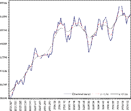
we want to emphasize the fact that holidays produce missing values in the series, but that does not prevent us from obtaining the trend with the data available. This is so because we use the Kalman filter to perform the calculations. In fact, all we need to do to get the estimated trend values for missing data is to skip the filter step in the Kalman filter recursions. The period of observation is the same as in the previous CETES28 example; hence, the values are also the same as in that exercise. We present the resulting estimated trend in Figure 8.

Figure 8. Daily IPC index and trends with 65% (=1.84) and 85% (=11.60) smoothness.
![]()
![]() The following application makes use of intraday data on the IPC. The
frequency of observation of the series is every 5min, from 8:30 a.m. to 3 p.m.
while the Mexican Stock Exchange is open. The sample period runs from April 17,
2006 to May 12, 2006 (19 working days), hence, the daily number of observations
is 78, for a total number of 1482 5-minute observations. To obtain the
smoothing constants for the trend we first obtained the values for N =19 days from Table II. These
values are =2.079 and 16.040 for percentages of
smoothness of 65 and 85%, respectively. The equivalent smoothing constants for
the series of 5-minute observations are obtained from the relation the
smoothing constant previously obtained. The resulting values are 12 for 65 and
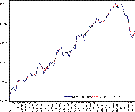
85%, respectively. In Figure 9 we appreciate the smooth curve representing the
trend, which behaves as the dynamic mean of the series and provides a nice
visual representation of the data.
The following application makes use of intraday data on the IPC. The
frequency of observation of the series is every 5min, from 8:30 a.m. to 3 p.m.
while the Mexican Stock Exchange is open. The sample period runs from April 17,
2006 to May 12, 2006 (19 working days), hence, the daily number of observations
is 78, for a total number of 1482 5-minute observations. To obtain the
smoothing constants for the trend we first obtained the values for N =19 days from Table II. These
values are =2.079 and 16.040 for percentages of
smoothness of 65 and 85%, respectively. The equivalent smoothing constants for
the series of 5-minute observations are obtained from the relation the
smoothing constant previously obtained. The resulting values are 12 for 65 and
85%, respectively. In Figure 9 we appreciate the smooth curve representing the
trend, which behaves as the dynamic mean of the series and provides a nice
visual representation of the data.
In this paper we propose to choose the smoothing constant of the ES filter with a method that arises by defining an index of smoothness that measures the relative precision of the smoothness component in the statistical model underlying the filter. The smoothing constant is shown to be a function of the desired percentage of smoothness for the trend, the sample size and the periodicity of the series. We could not get a closed expression of the smoothing constant, but we were able to provide an approximating formula with empirical support. Once the smoothing constant is chosen,

Figure 9. Intraday IPC index and trends with 65% (=162.16) and 85% (=1251.12) smoothness.
we suggest employing the Kalman filter to perform the required calculations for estimating the trend; thus, avoiding numerical problems that may arise from inverting large dimensional matrices.
We show that the procedure for choosing the smoothing constant of a daily time series can be generalized to time series with other than daily periodicities. The expression that relates equivalent smoothing constants is very simple for both series of flows or stocks. We also provide some evidence on the empirical benefits of using the daily frequency of observation as standard basis of reference. Thus, we consider the problem of obtaining the trend for the same time series observed with different periodicities. In that case, we show with some empirical examples that trends with equal degrees of smoothness, for different periodicities, show essentially the same dynamic behavior.
We illustrate the kind of results that can be obtained in practical applications by way of numerical examples. In particular, we consider situations in which the trend is needed for time series with lower than daily frequency or with intraday data. In those cases we show explicitly how to calculate the corresponding smoothing constant, starting from the equivalent daily one. Another situation of practical importance occurs when a time series has missing data, and we illustrate how that fact does not pose any problem for obtaining the trend. Another illustration allows us to see that obtaining trends for the same time series, but with different sample sizes, produces very similar numerical results.
Уважаемый посетитель!
Чтобы распечатать файл, скачайте его (в формате Word).
Ссылка на скачивание - внизу страницы.