Data with intraday frequency of observation have become
common use in finance due to the advances in data acquisition and storage.
Therefore, one objective of this work is to produce a method for trend
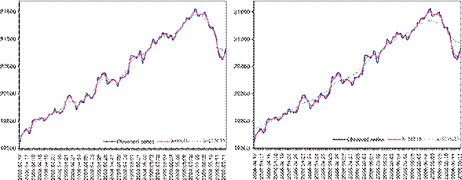
estimation of time series with intraday periodicity. In Figure 6 we plot the
trend of the intraday Mexican Stock Exchange index, named IPC (which is
Mexico’s most important financial index) with 55 and 65% smoothness and daily
and weekly base periodicities. The sample period runs from April 17, 2006 to
May 12, 2006, and covers N =19
days, so that =1.104 for S%![]() 079 for S%=65%. There are 78 observations
per day, so for daily data we get k=
079 for S%=65%. There are 78 observations
per day, so for daily data we get k=
![]() 78= S%=55%
and
78= S%=55%
and ![]() 162.162 for S%=65%. For this sample period
there are N =3
complete 5-day weeks, thus Table II indicates =3.025 for S%=55% and =13.375 for S%=65%.
Therefore, for a weekly basis we have k=
162.162 for S%=65%. For this sample period
there are N =3
complete 5-day weeks, thus Table II indicates =3.025 for S%=55% and =13.375 for S%=65%.
Therefore, for a weekly basis we have k=
![]() 390 75 for S%=55%, and
390 75 for S%=55%, and ![]() 25 for S%=65%. We did not use monthly or
quarterly periodicities because the resulting sample size became smaller than N
=1. It should be
clear from this example that
25 for S%=65%. We did not use monthly or
quarterly periodicities because the resulting sample size became smaller than N
=1. It should be
clear from this example that

Figure 6. Intraday IPC series and trends with: S%=55%, left: daily (=86.11) and weekly (=1179.75); S%=65%, right: daily (=162.16) and weekly (=5216.25).
estimated trends for series with weekly periodicity become too smooth for low percentages of smoothness. Moreover, it is not possible to obtain trends with a weekly basis and relatively high percentages of smoothness. For the aforementioned reasons we concluded that the most suitable basis periodicity is the daily one.
The proposed method is now applied to some of Mexico’s financial time series to illustrate different situations that may arise in practice.
![]()
![]()
![]()
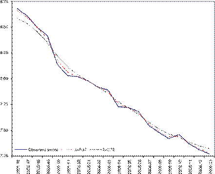
![]() In this illustration we estimate the trend of the weekly yield rate
of CETES28 employed previously (see Figure 5), but with different sample
periods. In fact, the sample period covers the third week of November, 2005 up
to the last week of March, 2006. We have to get first the ∗ value
of the weekly series equivalent to the constant used with the daily series. Since we are
dealing with a stock series, the equivalent smoothing constants are related by
100 daily data the values
that produce 65 and 85% smoothness of the trend are600, respectively.
Therefore, for the weekly series with n=20
we get 0.369 when S%=65% and 320 when S%=85%. The resulting trends are
shown in Figure 7. In particular, the trend with 85% smoothness shown in this
figure resembles closely that in Figure 5. This fact can be appreciated
numerically in Table IV. There we see that the trend figures are very close to
each other, mainly at the middle and the end of the shorter sample period.
In this illustration we estimate the trend of the weekly yield rate
of CETES28 employed previously (see Figure 5), but with different sample
periods. In fact, the sample period covers the third week of November, 2005 up
to the last week of March, 2006. We have to get first the ∗ value
of the weekly series equivalent to the constant used with the daily series. Since we are
dealing with a stock series, the equivalent smoothing constants are related by
100 daily data the values
that produce 65 and 85% smoothness of the trend are600, respectively.
Therefore, for the weekly series with n=20
we get 0.369 when S%=65% and 320 when S%=85%. The resulting trends are
shown in Figure 7. In particular, the trend with 85% smoothness shown in this
figure resembles closely that in Figure 5. This fact can be appreciated
numerically in Table IV. There we see that the trend figures are very close to
each other, mainly at the middle and the end of the shorter sample period.
We now use the method to obtain the trend for the daily 5-day week IPC index. This is a stock series whose period of observation runs from November 14, 2005 to March 31, 2006. In this case

Figure 7. Weekly yield rate of CETES28 and trends with S%=65% (=0.37) and S%=85% (=2.32).
![]() Table IV. Weekly yield
rate of CETES28. Selected trend values with S%=85%.
Table IV. Weekly yield
rate of CETES28. Selected trend values with S%=85%.
Sample used for trend estimation
|
Week |
Observed data |
2004:01–2006:13 |
2005:46–2006:13 |
|
2005:46 |
8.68 |
8.650 |
8.585 |
|
2005:47 |
8.61 |
8.569 |
8.534 |
|
2005:48 |
8.50 |
8.470 |
8.452 |
|
... |
... |
... |
... |
|
2006:01 |
7.98 |
7.979 |
7.978 |
|
2006:02 |
7.92 |
7.917 |
7.917 |
|
2006:03 |
7.89 |
7.854 |
7.853 |
|
... |
... |
... |
... |
|
2006:11 |
7.37 |
7.384 |
7.385 |
|
2006:12 |
7.31 |
7.345 |
7.346 |
|
2006:13 |
7.27 |
7.321 |
7.323 |
Уважаемый посетитель!
Чтобы распечатать файл, скачайте его (в формате Word).
Ссылка на скачивание - внизу страницы.