Simulink for beginners, страница 2

    [T,X,Y1,...,Yn] = SIM('model',TIMESPAN,OPTIONS,UT)

        T            : Returned time vector.

        X            : Returned state in matrix or structure format.

                       The state matrix contains continuous states followed by

                       discrete states.

        Y            : Returned output in matrix or structure format.

                       For block diagram models this contains all root-level

                       outport blocks.

        Y1,...,Yn    : Can only be specified for block diagram models, where n

                       must be the number of root-level outport blocks. Each

                       outport will be returned in the Y1,...,Yn variables.

        'model'      : Name of a block diagram model.

        TIMESPAN     : One of:

                         TFinal,

                         [TStart TFinal], or

                         [TStart OutputTimes TFinal].

                       OutputTimes are time points which will be returned in

                       T, but in general T will include additional time points.

        OPTIONS      : Optional simulation parameters. This is a structure

                       created with SIMSET using name value pairs.

        UT           : Optional extern input.  UT = [T, U1, ... Un]

                       where T = [t1, ..., tm]' or UT is a string containing a

                       function u=UT(t) evaluated at each time step.  For

                       table inputs, the input to the model is interpolated

                       from UT.

    Specifying any right hand side argument to SIM as the empty matrix, [],

    will cause the default for the argument to be used.

    Only the first parameter is required. All defaults will be taken from the

    block diagram, including unspecified options.  Any optional arguments

    specified will override the settings in the block diagram.

    See also SLDEBUG, SIMSET.

 Overloaded methods

    help network/sim.m

The simplest way to start is to use sim command in the following way.

» [t,x,y]=sim('untitled');

Next you can use plot command to see the result.

» plot(t,x)

To see y, you need to introduce an output in the SIMULINK model. Check below.

Another issue that we have not considered is initial condition. As you know every differential equation should have initial conditions given. The default value in SIMULINK is zero. To change that click the integrator. You’ll see the following display.

As seen above you can change the initial value to e.g. –3.

The default time for simulation is 10. If you wish to simulate longer you have to change it. To do that open Simulation menu and choose Simulation parameters.

You can change the Stop time according to your needs.

Complete the exercise. Run the simulation from SIMULINK and also from Command window.

DAMPED OSCILLATOR

Solve the damped oscillator problem

Assume that u(t) = 0, that is, there is no input.

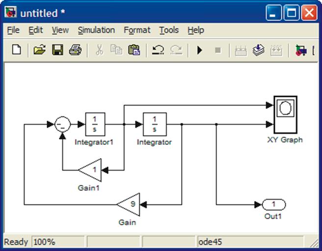
PURPOSE: To illustrate how to configure a SIMULINK diagram for a higher order differential equation and how to introduce initial conditions into it.

SOLUTION: Solve equation first with respect to the highest order derivative to obtain

To set up the right-hand side two integrators are needed:

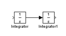
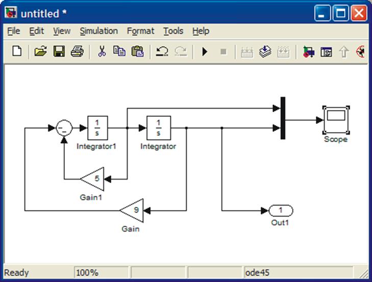
The input to the first integraror is the second derivative  and its output is . The latter is the innput to the second integrator producing x(t) at its output. In this way we have constructed the left-hand side of the equation. Since the second derivative  is equal to the right hand side, we collect it term by term. In order to do that we need   from the output of the first integrator, x(t) from the output of the second integrator and u(t), the step input must be generated. Here x(t) must also be multiplied by 9, so a gain is required. All these items are to be summed up so a sum block is also needed. The final configuration is given below. The initial values are added to the integrators. The resulting configuration is given below.

Next, set up the initial conditions by clicking the integrators one at a time and making appropriate changes.

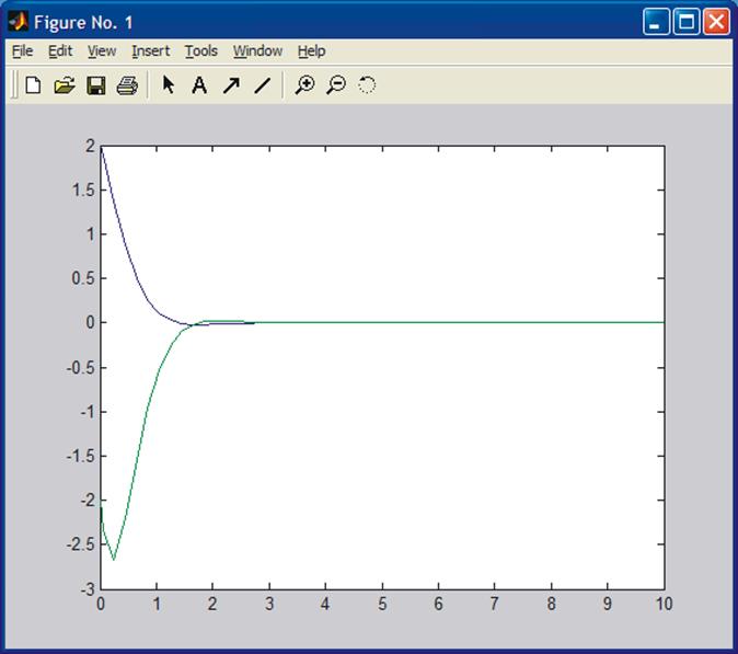
The solution x(t) and  are shown in Fig. below. The first figure is SIMULINK scope and the second is the result from Command window simulation.

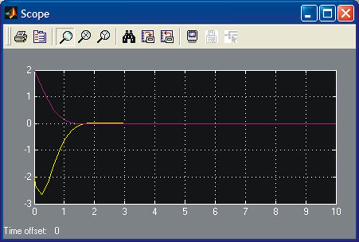
The sharpness of the lower curve around t = 0.4 s is not real, it should be smooth. First you might suspect numerical difficulties (there are none) due to too large a step size. This is not the case. It is due to display graphics, i.e., not enough points have been saved to have a smooth presentation.

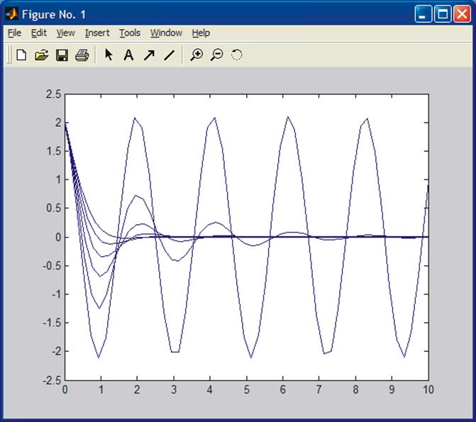
The damping factor can be changed by changing the coefficient 5 in front of . If the coefficient is zero (no damping), the result is a sinusoidal. Increasing the damping will result in damping oscillations. Complete the study to obtain the following responses.

Let us also plot a phase plane plot (x vs dx/dt). Note that here time has been eliminated. To see the effect better, start with less damping. Change the coefficient 5 to 1.

The result is shown below.

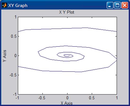
XY Graph does not adjust the scales automatically. In order to see the whole picture, click the XY Graph open and adjust the scales. Adjusting also the Sample time results in smooth picture.

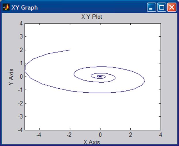
CONCLUSION: A stable system. It converges towards the origin. Physical interpretation: In origin both position and velocity are zero.