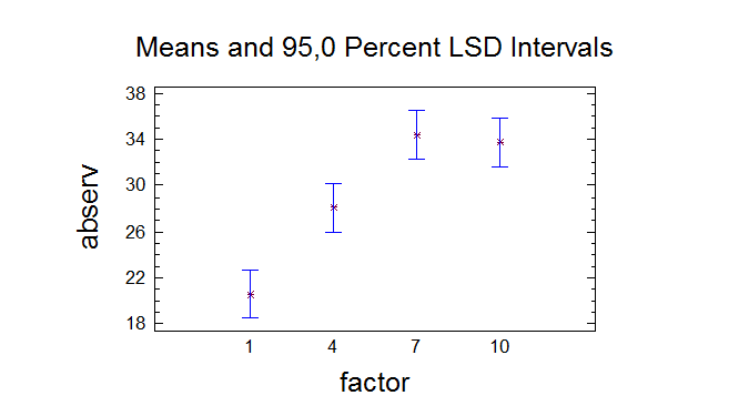
constructed in such a way that if two means are the same, their
intervals will overlap 95,0% of the time. You can display the
intervals graphically by selecting Means Plot from the list of
Graphical Options. In the Multiple Range Tests, these intervals are
used to determine which means are significantly different from which
others.
Multiple Range Tests for abserv by factor
-------------------------------------------------------------------------------Method: 95,0 percent LSD
factor Count Mean Homogeneous Groups
-------------------------------------------------------------------------------1 15 20,6 X
4 15 28,0667 X
10 15 33,7333 X
7 15 34,4 X
-------------------------------------------------------------------------------Contrast Difference +/- Limits
-------------------------------------------------------------------------------1 - 4 *-7,46667 4,23721
1 - 7 *-13,8 4,23721
1 - 10 *-13,1333 4,23721
4 - 7 *-6,33333 4,23721
4 - 10 *-5,66667 4,23721
7 - 10 0,666667 4,23721
-------------------------------------------------------------------------------* denotes a statistically significant difference.
The StatAdvisor
--------------This table applies a multiple comparison procedure to determine
which means are significantly different from which others. The bottom
half of the output shows the estimated difference between each pair of
means. An asterisk has been placed next to 5 pairs, indicating that
these pairs show statistically significant differences at the 95,0%
confidence level. At the top of the page, 3 homogenous groups are
identified using columns of X's. Within each column, the levels
containing X's form a group of means within which there are no
statistically significant differences. The method currently being
used to discriminate among the means is Fisher's least significant
difference (LSD) procedure. With this method, there is a 5,0% risk of
calling each pair of means significantly different when the actual
difference equals 0.
Variance Check
Cochran's C test: 0,450011 P-Value = 0,0500445
Bartlett's test: 1,56229 P-Value = 0,0000220176
Hartley's test: 17,0484
Levene's test: 7,21208 P-Value = 0,000354849
The StatAdvisor
--------------The four statistics displayed in this table test the null
hypothesis that the standard deviations of abserv within each of the 4
levels of factor is the same. Of particular interest are the three
P-values. Since the smallest of the P-values is less than 0,05, there
is a statistically significant difference amongst the standard
deviations at the 95,0% confidence level. This violates one of the
important assumptions underlying the analysis of variance and will
invalidate most of the standard statistical tests.
Kruskal-Wallis Test for abserv by factor
factor Sample Size Average Rank
-----------------------------------------------------------1 15 10,3333
4 15 29,6667
7 15 41,4333
10 15 40,5667
-----------------------------------------------------------Test statistic = 31,0727 P-Value = 8,20627E-7
The StatAdvisor
--------------The Kruskal-Wallis test tests the null hypothesis that the medians
of abserv within each of the 4 levels of factor are the same. The
data from all the levels is first combined and ranked from smallest to
largest. The average rank is then computed for the data at each
level. Since the P-value is less than 0,05, there is a statistically
significant difference amongst the medians at the 95,0% confidence
level. To determine which medians are significantly different from
which others, select Box-and-Whisker Plot from the list of Graphical
Options and select the median notch option.
Уважаемый посетитель!
Чтобы распечатать файл, скачайте его (в формате Word).
Ссылка на скачивание - внизу страницы.