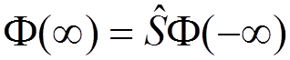
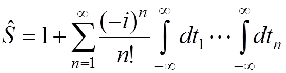
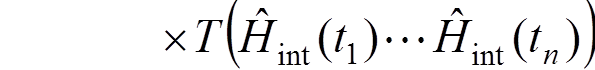
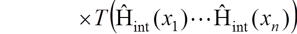
This equation can be solved by the iteration
procedure:
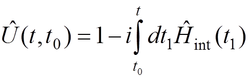
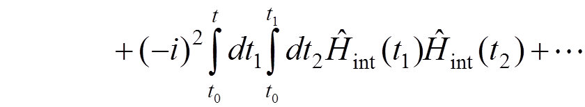
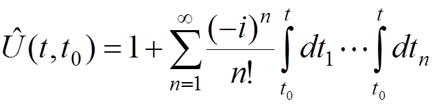
 ,
,
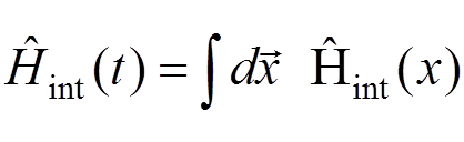
where ![]() is the time-ordered product operator.
is the time-ordered product operator.
This
expansion provides a basis for QED calculations by perturbation theory in  .
.
S-matrix and Green’s functions
We define the S-matrix by
 .
.
It
connects the state  and the state
  by
by
 .
.
The
perturbation expansion for ![]() :
:
 ,
,
where we have used
 .
.
This
expression for ![]() can be used for calculations of
scattering amplitudes for free particles
can be used for calculations of
scattering amplitudes for free particles  .
.
For processes involving bound states, one should use the corresponding expressions for so-called Green’s functions or other methods.
In particular, for a one-electron atom, the Green function can be defined by
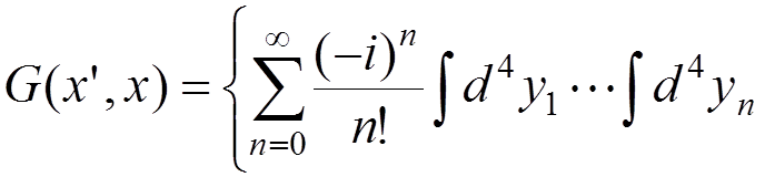
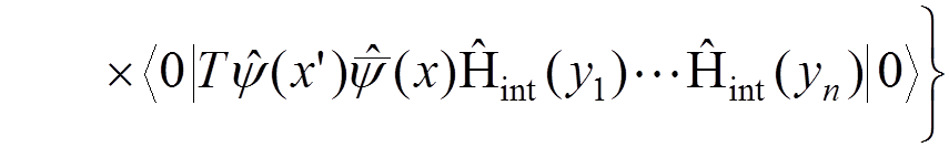
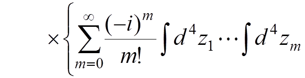
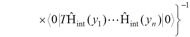 .
.
The
Green function 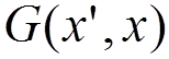 contains the total information about the energy levels of
the atom and can be calculated by perturbation theory according to its
definition. There are various mathematical methods to extract the energy levels
from
contains the total information about the energy levels of
the atom and can be calculated by perturbation theory according to its
definition. There are various mathematical methods to extract the energy levels
from
Feynman diagrams
The
calculations of ![]() and are performed using the expressions for
the field operators
and are performed using the expressions for
the field operators  ,
,  , and
, and
 in terms of the creation and annihilation
operators and the corresponding commutation relations.
in terms of the creation and annihilation
operators and the corresponding commutation relations.
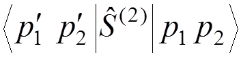
For instance, if we want to calculate the electron-electron scattering to the lowest order of the perturbation theory, we have to evaluate
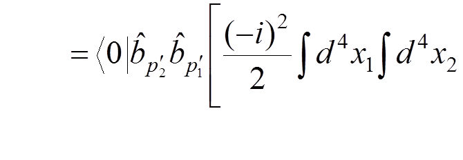
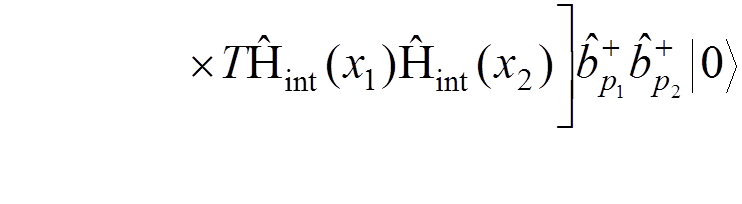

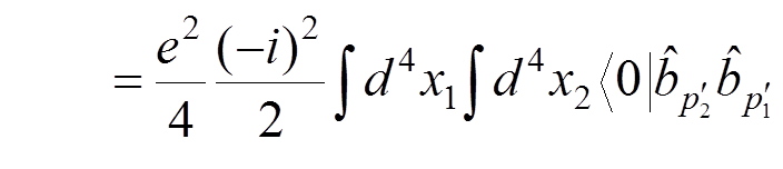

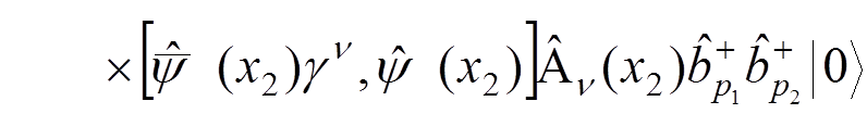 .
.
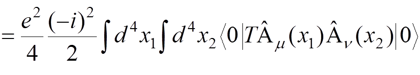
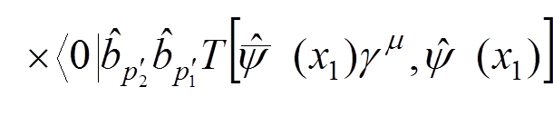
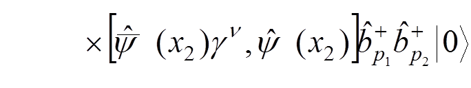 .
.
Denoting
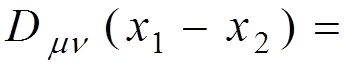
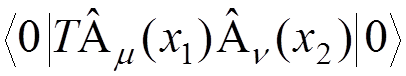
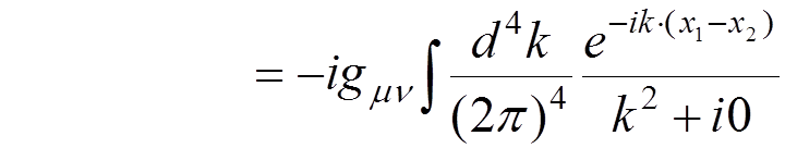 ,
,
that is
known as the photon
propagator, and
calculating the second factor, we obtain 
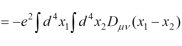
![]()

where 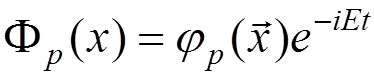 .
.
This expression can be represented by two Feynman diagrams
![]()
![]()
![]()
![]()
![]()

![]()
![]()
![]()
![]()
![]()
![]()

![]()
The diagram representation can be employed for every term of the perturbation expansion, if we formulate the following correspondence rules (Feynman’s rules):
1) Internal photon line
![]()


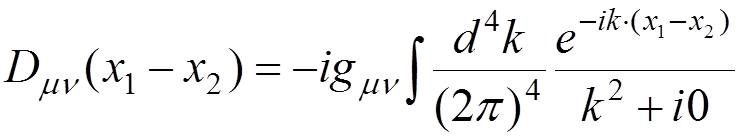
![]()
2) Internal electron line

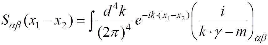
![]()
![]()
3) Vertex
![]()
![]()
![]()
![]()
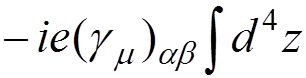
![]()
![]()


![]()
![]()
![]()
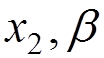
4) Incoming and outgoing electron lines


Outgoing
positron with 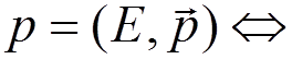 incoming electron with
 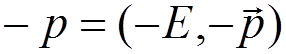 .
.
Incoming
positron with outgoing electron with .
5)
Symmetry
factor 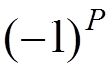 , where
 ![]() is the
parity of the permutation of the outgoing particles with respect to the
incoming ones.
is the
parity of the permutation of the outgoing particles with respect to the
incoming ones.
6) Factor  for every closed electron loop.
Similar Feynman’s rules can be formulated for Green’s functions.
It turns out that contributions of some diagrams are divergent at high internal momenta (small distances).
It can be shown that a one-loop diagram can be divergent only if
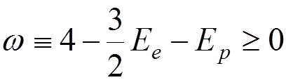 ,
,
where  is the number of external electron
lines,
is the number of external electron
lines, 
is the number of external photon lines.
Example:

![]()
![]()
![]()
Уважаемый посетитель!
Чтобы распечатать файл, скачайте его (в формате Word).
Ссылка на скачивание - внизу страницы.