Sparse Model Matrices
R Core Development Team
July 2007, 2008 (typeset on September 3, 2012)
Model matrices in the very widely used (generalized) linear models of statistics, (typically fit via lm() or glm() in R) are often practically sparse — whenever categorical predictors, factors in R, are used.
We show for a few classes of such linear models how to construct sparse model matrices using sparse matrix (S4) objects from the Matrix package, and typically without using dense matrices in intermediate steps.
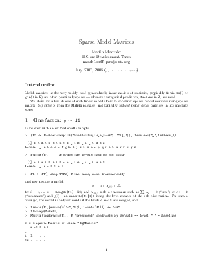
Let’s start with an artifical small example:
> (ff <- factor(strsplit("statistics_is_a_task", "")[[1]], levels=c("_",letters)))
[1] s t a t i s t i c s _ i s _ a _ t a s k
Levels: _ a b c d e f g h i j k l m n o p q r s t u v w x y z
> factor(ff) # drops the levels that do not occur
[1] s t a t i s t i c s _ i s _ a _ t a s k
Levels: _ a c i k s t
> f1 <- ff[, drop=TRUE] # the same, more transparently
and now assume a model yi = µ + αj(i) + Ei,
for i = 1,...,n = length(f1)= 20, and αj(i) with a constraint such as Pj αj = 0 (“sum”) or α1 = 0 (“treatment”) and j(i) =as.numeric(f1[i]) being the level number of the i-th observation. For such a “design”, the model is only estimable if the levels c and k are merged, and
> levels(f1)[match(c("c","k"), levels(f1))] <- "ck"
> library(Matrix)
> Matrix(contrasts(f1)) # "treatment" contrasts by default -- level "_" = baseline
6 x 5 sparse Matrix of class "dgCMatrix" a ck i s t _ . . . . . a 1 . . . . ck . 1 . . .
i . . 1 . .
s . . . 1 .
t . . . . 1
> Matrix(contrasts(C(f1, sum))) 6 x 5 sparse Matrix of class "dgCMatrix"
_ 1 . . . .
a . 1 . . . ck . . 1 . .
i . . . 1 .
s . . . . 1 t -1 -1 -1 -1 -1
> Matrix(contrasts(C(f1, helmert)), sparse=TRUE) # S-plus default; much less sparse
6 x 5 sparse Matrix of class "dgCMatrix"
_ -1 -1 -1 -1 -1 a 1 -1 -1 -1 -1 ck . 2 -1 -1 -1 i . . 3 -1 -1
s . . . 4 -1
t . . . . 5
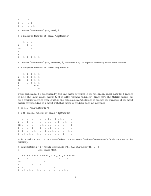
where contrasts() is (conceptually) just one major ingredient in the well-known model.matrix() function to build the linear model matrix X of so-called “dummy variables”. Since 2007, the Matrix package has been providing coercion from a factor object to a sparseMatrix one to produce the transpose of the model matrix corresponding to a model with that factor as predictor (and no intercept):
> as(f1, "sparseMatrix")
6 x 20 sparse Matrix of class "dgCMatrix"
_ . . . . . . . . . . 1 . . 1 . 1 . . . .
a . . 1 . . . . . . . . . . . 1 . . 1 . . ck . . . . . . . . 1 . . . . . . . . . . 1 i . . . . 1 . . 1 . . . 1 . . . . . . . . s 1 . . . . 1 . . . 1 . . 1 . . . . . 1 .
t . 1 . 1 . . 1 . . . . . . . . . 1 . . .
which is really almost the transpose of using the above sparsification of contrasts() (and arranging for nice printing),
> printSpMatrix( t( Matrix(contrasts(f1))[as.character(f1) ,] ),
+ col.names=TRUE)
s t a t i s t i ck s _ i s _ a _ t a s cka . . 1 . . . . . . . . . . . 1 . . 1 . . ck . . . . . . . . 1 . . . . . . . . . . 1 i . . . . 1 . . 1 . . . 1 . . . . . . . . s 1 . . . . 1 . . . 1 . . 1 . . . . . 1 .
t . 1 . 1 . . 1 . . . . . . . . . 1 . . .
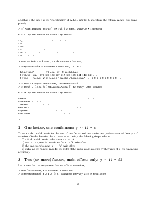
and that is the same as the “sparsification” of model.matrix(), apart from the column names (here transposed),
> t( Matrix(model.matrix(~ 0+ f1))) # model with*OUT* intercept
6 x 20 sparse Matrix of class "dgCMatrix"
f1_ . . . . . . . . . . 1 . . 1 . 1 . . . . f1a . . 1 . . . . . . . . . . . 1 . . 1 . . f1ck . . . . . . . . 1 . . . . . . . . . . 1 f1i . . . . 1 . . 1 . . . 1 . . . . . . . . f1s 1 . . . . 1 . . . 1 . . 1 . . . . . 1 . f1t . 1 . 1 . . 1 . . . . . . . . . 1 . . .
A more realistic small example is the chickwts data set,
> str(chickwts)# a standard R data set, 71 x 2
'data.frame': 71 obs. of 2 variables:
$ weight: num 179 160 136 227 217 168 108 124 143 140 ...
$ feed : Factor w/ 6 levels "casein","horsebean",..: 2 2 2 2 2 2 2 2 2 2 ...
> x.feed <- as(chickwts$feed, "sparseMatrix")
> x.feed[ , (1:72)[c(TRUE,FALSE,FALSE)]] ## every 3rd column:
6 x 24 sparse Matrix of class "dgCMatrix"
casein . . . . . . . . . . . . . . . . . . . . 1 1 1 1 horsebean 1 1 1 1 . . . . . . . . . . . . . . . . . . . . linseed . . . . 1 1 1 1 . . . . . . . . . . . . . . . . meatmeal . . . . . . . . . . . . . . . . 1 1 1 1 . . . . soybean . . . . . . . . 1 1 1 1 . . . . . . . . . . . . sunflower . . . . . . . . . . . . 1 1 1 1 . . . . . . . .
>
To create the model matrix for the case of one factor and one continuous predictor—called “analysis of covariance” in the historical literature— we can adopt the following simple scheme.
The final model matrix is the concatenation of:
1) create the sparse 0-1 matrix m1 from the f1 main-effect
2) the single row/column ’x’ == ’x’ main-effect
3) replacing the values 1 in m1@x (the x-slot of the factor model matrix), by the values of x (our continuous predictor).
Let us consider the warpbreaks data set of 54 observations,
> data(warpbreaks)# a standard R data set
> str(warpbreaks) # 2 x 3 (x 9) balanced two-way with 9 replicates:
'data.frame': 54 obs. of 3 variables:
$ breaks : num 26 30 54 25 70 52 51 26 67 18 ...
$ wool : Factor w/ 2 levels "A","B": 1 1 1 1 1 1 1 1 1 1 ...
$ tension: Factor w/ 3 levels "L","M","H": 1 1 1 1 1 1 1 1 1 2 ...
> xtabs(~ wool + tension, data = warpbreaks)
tension
wool L M H A 9 9 9
B 9 9 9
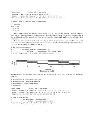
This example depicts how a model matrix would be built for the model breaks wool + tension. Since this is a main effects model (no interactions), the desired model matrix is simply the concatenation of the model matrices of the main effects. There are two here, but the principle applies to general main effects of factors.
The most sparse matrix is reached by not using an intercept, (which would give an all-1-column) but rather have one factor fully coded (aka“swallow”the intercept), and all others being at "treatment" contrast, i.e., here, the transposed model matrix, tmm, is
> tmm <- with(warpbreaks,
+ rBind(as(tension, "sparseMatrix"),
+ as(wool, "sparseMatrix")[-1,,drop=FALSE]))
> print( image(tmm) ) # print(.) the lattice object

10 20 30 40 50
Column
Dimensions: 4 x 54
The matrices are even sparser when the factors have more than just two or three levels, e.g., for the morley data set,
> data(morley) # a standard R data set
> morley$Expt <- factor(morley$Expt)
> morley$Run <- factor(morley$Run) > str(morley)
'data.frame': 100 obs. of 3 variables:
$ Expt : Factor w/ 5 levels "1","2","3","4",..: 1 1 1 1 1 1 1 1 1 1 ...
$ Run : Factor w/ 20 levels "1","2","3","4",..: 1 2 3 4 5 6 7 8 9 10 ... $ Speed: int 850 740 900 1070 930 850 950 980 980 880 ...
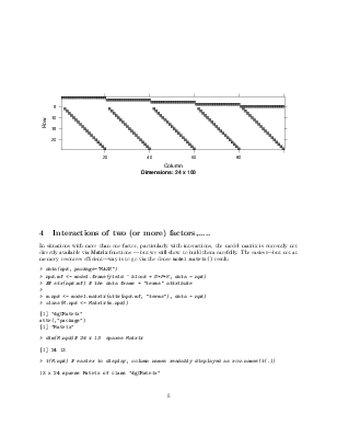
> t.mm <- with(morley,
+ rBind(as(Expt, "sparseMatrix"),
+ as(Run, "sparseMatrix")[-1,]))
> print( image(t.mm) ) # print(.) the lattice object
Column
Dimensions: 24 x 100
4 Interactions of two (or more) factors,.....
In situations with more than one factor, particularly with interactions, the model matrix is currently not directly available via Matrix functions — but we still show to build them carefully. The easiest—but not at memory resources efficient—way is to go via the dense model.matrix() result:
> data(npk, package="MASS")
> npk.mf <- model.frame(yield ~ block + N*P*K, data = npk)
> ## str(npk.mf) # the data frame + "terms" attribute
>
> m.npk <- model.matrix(attr(npk.mf, "terms"), data = npk)
> class(M.npk <- Matrix(m.npk))
[1] "dgCMatrix" attr(,"package") [1] "Matrix"
> dim(M.npk)# 24 x 13 sparse Matrix
[1] 24 13
> t(M.npk) # easier to display, column names readably displayed as row.names(t(.))
13 x 24 sparse Matrix of class "dgCMatrix"
(Intercept) 1 1 1 1 1 1 1 1 1 1 1 1 1 1 1 1 1 1 1 1 1 1 1 1
|
block2 |
. . . . 1 1 1 1 . . . . . . . . . . . . . . . . |
|
block3 |
. . . . . . . . 1 1 1 1 . . . . . . . . . . . . |
|
block4 |
. . . . . . . . . . . . 1 1 1 1 . . . . . . . . |
|
block5 |
. . . . . . . . . . . . . . . . 1 1 1 1 . . . . |
|
block6 |
. . . . . . . . . . . . . . . . . . . . 1 1 1 1 |
|
N1 |
. 1 . 1 1 1 . . . 1 1 . 1 1 . . 1 . 1 . 1 1 . . |
|
P1 |
1 1 . . . 1 . 1 1 1 . . . 1 . 1 1 . . 1 . 1 1 . |
|
K1 |
1 . . 1 . 1 1 . . 1 . 1 . 1 1 . . . 1 1 1 . 1 . |
|
N1:P1 |
. 1 . . . 1 . . . 1 . . . 1 . . 1 . . . . 1 . . |
|
N1:K1 |
. . . 1 . 1 . . . 1 . . . 1 . . . . 1 . 1 . . . |
|
P1:K1 |
1 . . . . 1 . . . 1 . . . 1 . . . . . 1 . . 1 . |
|
N1:P1:K1 |
. . . . . 1 . . . 1 . . . 1 . . . . . . . . . . |
Another example was reported by a user on R-help (July 15, 2008, https://stat.ethz.ch/pipermail/ r-help/2008-July/167772.html) about an “aov error with large data set”.
’m looking to analyze a large data set: a within-Ss 2*2*1500 design with 20 Ss. However, aov() gives me an error.
And gave the following code example (slightly edited):
> id <- factor(1:20)
> a <- factor(1:2)
> b <- factor(1:2)
> d <- factor(1:1500)
> aDat <- expand.grid(id=id, a=a, b=b, d=d)
> aDat$y <- rnorm(length(aDat[, 1])) # generate some random DV data > dim(aDat
Уважаемый посетитель!
Чтобы распечатать файл, скачайте его (в формате Word).
Ссылка на скачивание - внизу страницы.