Галушкин И. В. Е-441
Прикладная статистика.
Лабораторная работа № 9.
Регрессионный анализ в пакетах STATGRAPHICS и MATHCAD.
Вариант № 2:
|
x |
2.7 |
4.6 |
6.3 |
7.8 |
9.2 |
10.6 |
12.0 |
13.4 |
14.7 |
|
y |
17.0 |
16.2 |
13.3 |
13.0 |
9.7 |
9.9 |
6.2 |
5.8 |
5.7 |
STATGRAPHICS:
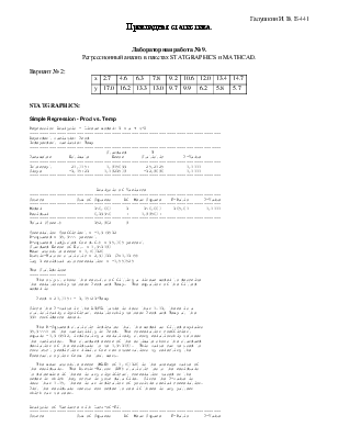
Simple Regression - Prod vs. Temp
Regression Analysis - Linear model: Y = a + b*X
----------------------------------------------------------------------------Dependent variable: Prod
Independent variable: Temp
----------------------------------------------------------------------------Standard T
Parameter Estimate Error Statistic P-Value
----------------------------------------------------------------------------Intercept 20,3057 0,805699 25,2025 0,0000
Slope -1,05721 0,0821538 -12,8686 0,0000
----------------------------------------------------------------------------Analysis of Variance
----------------------------------------------------------------------------Source Sum of Squares Df Mean Square F-Ratio P-Value
----------------------------------------------------------------------------Model 146,663 1 146,663 165,60 0,0000
Residual 6,19946 7 0,885637
----------------------------------------------------------------------------Total (Corr.) 152,862 8
Correlation Coefficient = -0,979512
R-squared = 95,9444 percent
R-squared (adjusted for d.f.) = 95,365 percent
Standard Error of Est. = 0,941083
Mean absolute error = 0,763126
Durbin-Watson statistic = 2,93311 (P=0,0175)
Lag 1 residual autocorrelation = -0,553525
The StatAdvisor
--------------The output shows the results of fitting a linear model to describe
the relationship between Prod and Temp. The equation of the fitted
model is
Prod = 20,3057 - 1,05721*Temp
Since the P-value in the ANOVA table is less than 0.01, there is a
statistically significant relationship between Prod and Temp at the
99% confidence level.
The R-Squared statistic indicates that the model as fitted explains
95,9444% of the variability in Prod. The correlation coefficient
equals -0,979512, indicating a relatively strong relationship between
the variables. The standard error of the estimate shows the standard
deviation of the residuals to be 0,941083. This value can be used to
construct prediction limits for new observations by selecting the
Forecasts option from the text menu.
The mean absolute error (MAE) of 0,763126 is the average value of
the residuals. The Durbin-Watson (DW) statistic tests the residuals
to determine if there is any significant correlation based on the
order in which they occur in your data file. Since the P-value is
less than 0.05, there is an indication of possible serial correlation.
Plot the residuals versus row order to see if there is any pattern
which can be seen.
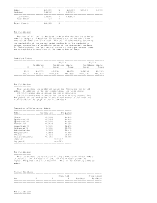
Analysis of Variance with Lack-of-Fit
----------------------------------------------------------------------------Source Sum of Squares Df Mean Square F-Ratio P-Value
----------------------------------------------------------------------------Model 146,663 1 146,663 165,60 0,0000
Residual 6,19946 7 0,885637
----------------------------------------------------------------------------Lack-of-Fit 6,19946 7 0,885637
Pure Error 0,0 0
----------------------------------------------------------------------------Total (Corr.) 152,862 8
The StatAdvisor
--------------The lack of fit test is designed to determine whether the selected
model is adequate to describe the observed data, or whether a more
complicated model should be used. The test is performed by comparing
the variability of the current model residuals to the variability
between observations at replicate values of the independent variable
X. Unfortunately, the test can not be run in this case because there
are no replicate observations at the same values of Temp.
Predicted Values
Уважаемый посетитель!
Чтобы распечатать файл, скачайте его (в формате Word).
Ссылка на скачивание - внизу страницы.