Compensation of disturbance for state-delayed plants, страница 2

where estimation vector is produced by observer  (7),(8), vector is constant coefficients vector, and function  is exponentially fading.

Theorem proving

Let nullity vector is defined as

               .                                                                                 (11)

Subject to (1, 7-11), differentiated nullity vector looks like:

         (12)

Since matrix G is defined as hurwitz, vector  at .

               3.2 Synthesis of control law.

We have a purpose to stabilize the plant by compensation of external disturbance.

To make this, let’s choose the control law in a following way:

,                                                                                         (13)

where vector  is  adjustable parameters vector, which adjusting algorithm will be defined further, vector  is produced by observer (7),(8).  Coefficient and matrix  will be defined further. Vector k is choosing in such way, that matrix  will be stable.

Now we must define adjusting algorithm , conditions for choosing coefficientand matrixfor synthesis necessary control signal, which will provide fulfillment of condition .

The functional Lyapunov-Krasovsky for these conditions can be presented in such form:

,                                                       (14)

where  - is some symmetrical positive defined matrix (it will be defined further), is some positive coefficient.

Derivative from this functional along trajectory of the plant (1), taking into account (10) and (14), (vector  is neglected as tending to zero) looks like:

                                           (15)

For system (1),(2) asymptotic stability, the fulfillment of following condition is necessary:

,                                                                                                  (16)

where Q is some symmetrical positive defined matrix.

To simplify a functional derivative expression, let’s use known estimation.

,                                                                     (17)

Since matrix D  can be parameterized as , expression (17) can be transformed:

                                    (18)

where - constant coefficient.

We can find a following expression for functional derivative putting into derivative expression (15) obtained estimation (17),(18), and control signal  u (13):

,                      (19)

where I is identity matrix suitable dimension.

Let’s choose adjusting algorithm in following way:

.                                                                                                          (20)

So we can find out such expression:         

.                                                    (21)

To comply the target conditions, we have to complete this inequation:

                                      (22)

A condition  has to be fulfilled, at the same time matrix P must be found from Lyapunov equation:

.                                                                                             (23)

Thus, we’ve got all conditions for all needed parameters of control law, which are necessary for plant stabilization.

4. System example

An example of control system simulation with all mentioned hypotheses is given below

A plant is given by an equation

, , ,

Disturbance will be defined as sustained vibrations,.

It represents primitive integral of differential equation  with initial conditions , , i.e. it can be considered as output of linear generator:

,  , .

Pair (G,l) must be fully controlled and matrix G must be hurwitz. So, (G,l) can be presented as

, .

Matrix N has to satisfy the condition (9), therefore (b=l) we will choose is as .

Value of coefficienthas no matter for external disturbance compensation, but it exerts a great influence on the transient performance. As we have not to achieve defined quality index in this example, we can put any value of this coefficient. Let.

For this matrix D, coefficient 1.26. Value of coefficient  has to satisfy condition (25), it is important to mark, that it also has influence on transient performance.

For this example, let  and .

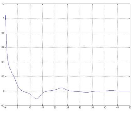
The results of such system modeling in simulink environment with initial data mentioned previously are given below. Transient performance for first component of vector x looks like:

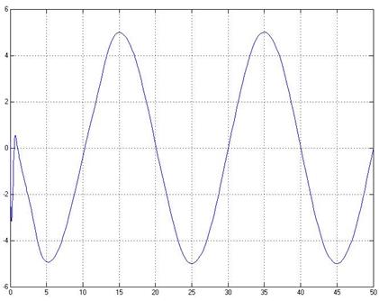
After a time, the control signal u(t) begins  to reproduce disturbance f , but with opposite sign. Vector x tends to zero.  It looks like:

              

5. Conclusion

Thus, we have formed an adaptive control system allowing to stabilize a plant with delay under external disturbance. At that, we have measured only state vector. We’ve used inner model method [1], extended for plants with time-delay. At the same time, all indeterminacy of disturbance  is taking to indeterminacy of vector . It’s noteworthy that control algorithm doesn’t depend on time of delay .

References

[1].  Nikiforov V.O.  «External determinant disturbance observers» Automatics and Telemechanics, 2004 #10 p.

13-24. (in Russian)

[2]. Miroshnik I.V., Nikiforov V.O., Fradkov A.L. “Nonlinear  and adaptive control of complex dynamical systems”, St. Petersburg: Nauka, 2000  (in Russian)

[3]. Kolmanovsky V.B., Nosov V.R. “Stability and periodical states of conrol systems with delay”, St. Petersburg: Nauka, 1981  (in Russian)