Convolution Matrices for Signal Processing Applications in MATLAB, страница 2

         0         0         0

         0         0         0

         0         0         0

         0         0         0

         0         0         0

         0         0         0

    0.0528         0         0

    0.2639    0.0528         0

    0.4944    0.2639    0.0528

y =

   -6.327476116625931e-003

   -3.508401686198939e-002

   -5.088287847879567e-002

    2.113359923355307e-002

    5.758050004475002e-002

   -1.556115559503205e-001

   -4.212745748596921e-001

   -2.825565027954645e-001

    2.945023636337310e-001

    6.022916921622209e-001

y1 =

   -6.327476116625931e-003

   -3.508401686198939e-002

   -5.088287847879567e-002

    2.113359923355305e-002

    5.758050004475004e-002

   -1.556115559503206e-001

   -4.212745748596921e-001

   -2.825565027954644e-001

    2.945023636337310e-001

    6.022916921622210e-001  

APPLICATION - DECONVOLUTION

Deconvolution is the operation of reconstructing the input to a system, given a description of the system and the output.

 

Given y(n) and H, find x(n).

An example of this problem is: given the average weekly temperatures throughout the week, can we find the daily temperatures?

For now let's consider the filter b,a we defined up above.  As an example input, let's input a square pulse to the filter

         n = 30;            % length of input signal

         t = (0:n-1)';      % index vector     

         x = (t>5)&(t<15);  % a pulse at t = 6,7,8,... 14         

         y = filter(h,1,x);   

         clf, plot(t,x,t,y)

  

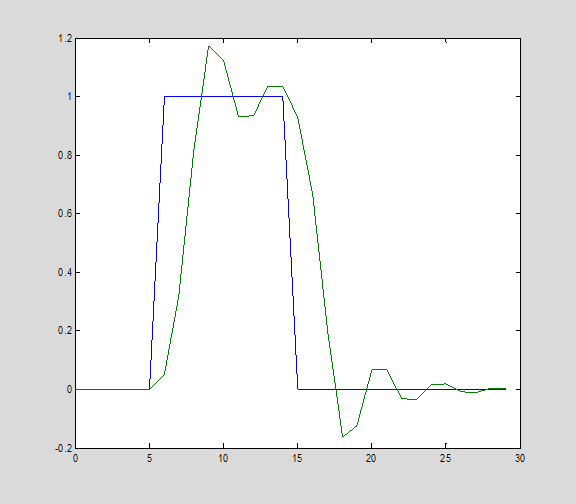
Notice that y is a 'smoothed' version of x.

For a length n signal, this filter's convolution matrix is

        C = convmtx(h,n);

        C = C(1:n,:);     % keep only first n rows (truncates output)         

A simple solution is to invert the matrix to recover the input x from the output y.  We use \ to get the least squares, or pseudo inverse, solution.

         x1 = C\y;

         plot(t,x,t,x1)         

     (This is equivalent to      x1 = pinv(C)*y;   )

  

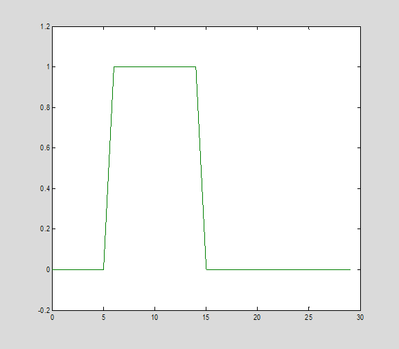
The input has been recovered EXACTLY now (provided the convolution matrix may be inverted).

DECONVOLUTION WITH ADDITIVE NOISE

Now consider the case where there is some noise added to the output of the system prior to the measurements.

					y(n)
		r(n)

Now the inversion process suffers from 'noise gain'.  For example, add some white noise to the output prior to inverting:

         r = randn(n,1)/100;

         x2 = pinv(C)*(y+r);

         plot(t,x,t,x2)         

  

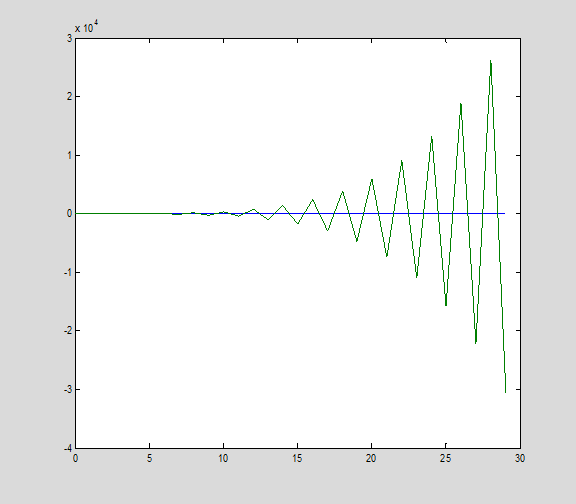
The deconvolved input has gone berserk!  Why is this?  We only added a bit of noise.  The reason is because some of the singular values of our matrix are very very small:

         s = svd(C);

         clf, plot(s)     

When we invert the output y+r, we multiply its coordinates in the basis of the singular vectors of C by the inverse of the singular values.

         clf, plot(1./s)       

  

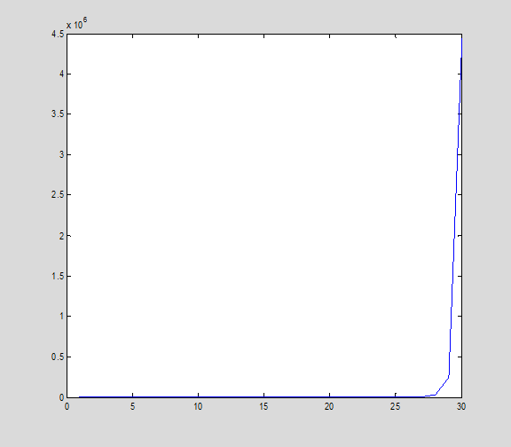
The last 5 or so singular values, when inverted, lead to a HUGE gain in the signal components in the span of those last singular vectors.

TRADING OFF NOISE GAIN FOR RESOLUTION

What can we do about noise gain?  We can truncate the inversion to exclude the last singular values that  are tiny. 

This can be done in the pinv function by passing a tolerance.  The pseudo inverse will treat all singular values less than the tolerance as zero.

         x2 = pinv(C,s(n-5))*(y+r);

         plot(t,x,t,x2)          

Here we've truncated the last five singular vectors.  We still see a lot of ringing, but the edges of the pulse are very exact.

         x2 = pinv(C,s(n-10))*(y+r);

         plot(t,x,t,x2)      

  

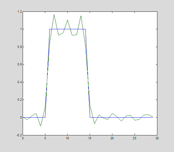
Taking away the last 10 singular vectors, the input pulse is very closely recovered.  The ringing is reduced, and the edges of the pulse are easy to distinguish.

         x2 = pinv(C,s(5))*(y+r);

         plot(t,x,t,x2)       

This time, taking away all but 5 singular values, we see very little noise effects but the pulse is smeared.  We have lost resolution but have also reduced noise gain.

TRY ME

Try this out with other filters, signal lengths, signals, and number of singular values retained.