Возможности среды Matlab для построения нейронных сетей, использование предоставленными возможностями, страница 5

P = {rands(5,4)};

[Y,Pf,Af] = sim(net,{4 50},{},P);

Y{end}

ans =

1     1     1    -1

1    -1    -1    -1

1    -1     1    -1

1     1     1     1

1    -1     1     1

Некоторые начальные условия ведут к желаемым стабильным точкам. другие ведут к неделательным стабильным точкам.

2.9. Примеры приложений

2.9.1.  Linear design

В отличие от большинства других архитектур сетей, линейные сети могут быть беспрепятственно спроектированы, если известны пары входных/целевых векторов. Можно получить конкретные значения сети для весов и порогов, чтобы минимизировать среднеквадратичную ошибку при помощи функции newlind.

%    NEWLIND - Solves for a linear layer.

%    SIM   - Simulates a linear layer.

%    LINEAR PREDICTION:

%    Using the above functions a linear neuron is designed

%    to predict the next value in a signal, given the last

%    five values of the signal.

pause % Strike any key to continue...

%    DEFINING A WAVE FORM

%    ====================

%    TIME defines the time steps of this simulation.

time = 0:0.025:5;  % from 0 to 6 seconds

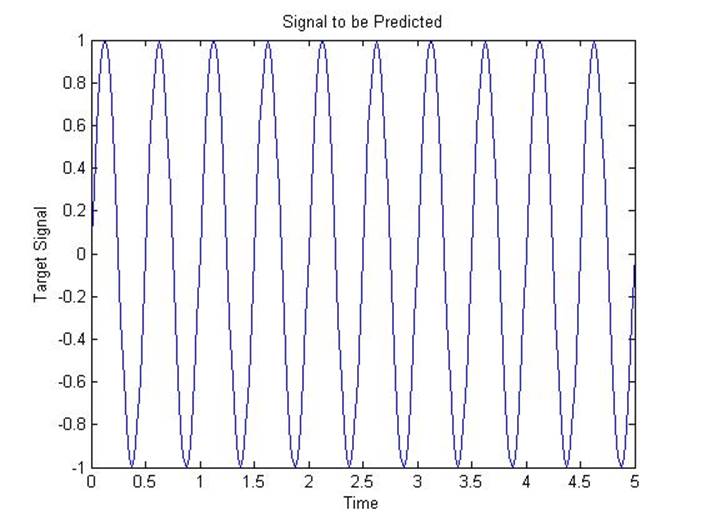
%    T defines the signal in time to be predicted:

T = sin(time*4*pi);

Q = length(T);

%    The input P to the network is the last five values

%    of the signal T:

P = zeros(5,Q);

P(1,2:Q) = T(1,1:(Q-1));

P(2,3:Q) = T(1,1:(Q-2));

P(3,4:Q) = T(1,1:(Q-3));

P(4,5:Q) = T(1,1:(Q-4));

P(5,6:Q) = T(1,1:(Q-5));

pause % Strike any key to see these signals...

%    PLOTTING THE SIGNALS

%    ====================

%    Here is a plot of the signal to be predicted:

plot(time,T)

xlabel('Time');

ylabel('Target Signal');

title('Signal to be Predicted');

pause % Strike any key to design the network...

%    NEWLIND solves for weights and biases which will let

%    the linear neuron model the system.

net = newlind(P,T);

pause % Strike any key to test the predictor...

%    TESTING THE PREDICTOR

%    =====================

%    SIM simulates the linear neuron which attempts

%    to predict the next value in the signal at each

%    timestep.

a = sim(net,P);

%    The output signal is plotted with the targets.

plot(time,a,time,T,'+')

xlabel('Time');

ylabel('Output -  Target +');

title('Output and Target Signals');

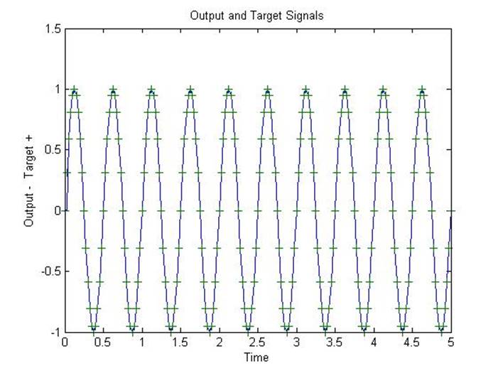
%    The linear neuron does a good job.

pause % Strike any key to see the error signal...

%    Error is the difference between output and target signals.

e = T - a;

%    This error can be plotted.

plot(time,e)

hold on

plot([min(time) max(time)],[0 0],':r')

hold off

xlabel('Time');

ylabel('Error');

title('Error Signal');

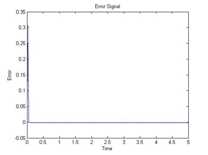
%    Notice how small the error is!

echo off

End of APPLIN1

2.9.2.  Adaptive linear prediction

В данной демонстрации линейная сеть обучается постепенно при помощи функции adapt, чтобы предугадывать временные ряды. Поскольку сеть обучается постепенно, она может реагировать на изменения в отношениях между прошлыми и будущими значениями сигнала.

%    NEWLIN  - Creates and initializes a linear layer.

%    ADAPT  - Trains a linear layer with Widrow-Hoff rule.

%    ADAPTIVE LINEAR PREDICTION:

%    Using the above functions a linear neuron is adaptively

%    trained to predict the next value in a signal, given the

%    last five values of the signal.

%    The linear neuron is able to adapt to changes in the

%    signal it is trying to predict.

pause % Strike any key to continue...

%    DEFINING A WAVE FORM

%    ====================

%    TIME1 and TIME2 define two segments of time.

time1 = 0:0.025:4;      % from 0 to 4 seconds

time2 = 4.05:0.025:6;  % from 4 to 6 seconds

%    TIME defines all the time steps of this simulation.

time = [time1 time2];  % from 0 to 6 seconds

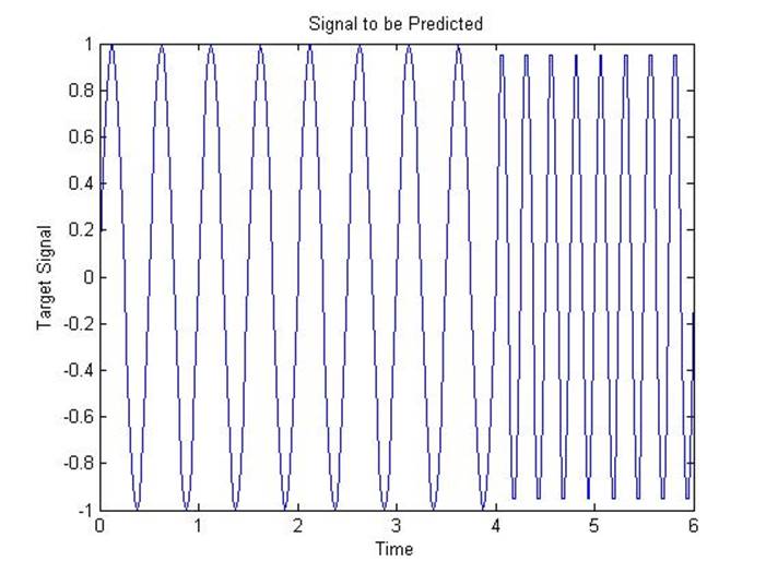
%    T defines a signal which changes frequency once:

T = con2seq([sin(time1*4*pi) sin(time2*8*pi)]);

%    The input P to the network is the same as the

%    target.  The network will use the last five

%    values of the target to predict the next value.

P = T;

pause % Strike any key to see these signals...

%    PLOTTING THE SIGNALS

%    ====================

%    Here is a plot of the signal to be predicted:

plot(time,cat(2,T{:}))

xlabel('Time');

ylabel('Target Signal');

title('Signal to be Predicted');