Limiting Surfaces. Limiting Surfaces Example. When surfaces are limited together PowerSHAPE automatically trims back the surfaces, страница 2

Double clicking on this surface will bring up the primitive options form. To modify the trimming the surface must be converted to a Power surface. Once converted, double-clicking will bring up new toolbars at the top of the screen.

·  From the Right Mouse Menu, select Convert Surface.

·  Double Click on thenew surface.

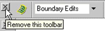
Two new toolbars appear under the edit toolbar.  These are surface edit and curve edit below. These toolbars can be closed by selecting the small ‘x’ on the left of each tool bar.

·  From the surface edit toolbar, select Enter trim Region Editing.

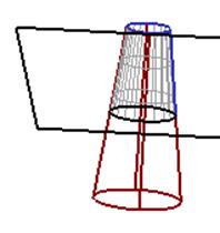
As soon as the trim region editing has been selected, the whole surface is shown, with the limited region shown in grids.

The Trim Region Edit toolbar appears.

·  Select boundary selector.

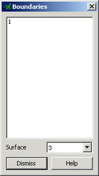
The boundary form appears which lists all of the available boundaries in the selected surface.

·  Select boundary 1 by clicking on the number 1.

·  Select Reverse the Boundary. 

The boundary on the cone has been reversed giving the other trimming option, which shows the bottom part of the surface.

·  Exit out of trimming mode by removing the trimming toolbar.

·  Select and Delete all surfaces.

Toy Submarine Example

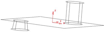
Surfaces do not have to be limited back to other surfaces; they can be limited back to intersection curves, Workplanes and geometry as this example shows.

·  Generatea sphere of radius 30 at the workplane.

·  From the Editing toolbar select Scale the object(s).

The scaling toolbar appears.

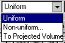·  Select the down arrow on Uniform to display the options.

If a scaling factor was required, the option uniform is used. With non-uniform you can specify different scale factors for different axis. Otherwise you can scale to a projected volume.

·  Select Non-uniform.

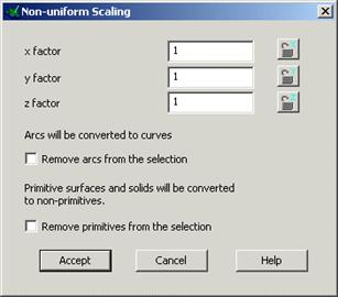
A form appears allowing the X, Y and Z values to be given separately. These can be input as decimal numbers i.e. 1.5 or as fractions i.e. 15/10. The form converts fractions to decimal numbers.

·  Enter 50/30 for x factor, 20/30 for y factor and 0.75 for z factor.

·  Press Accept. Select Shaded View.

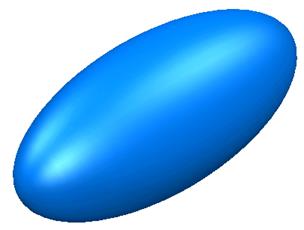
The sphere has been scaled down to a more oval shape. The shaded view has been selected to see the surface more clearly.

Note: If the general tolerance is changed you may have more internal curves shown in the wireframe view.

·  Create a cone at the workplane with a base radius 20, top radius 10 and length of 40.

·  Select transparent view.

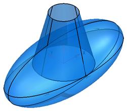
The transparent view shows inside the surfaces so you can see if surfaces have been trimmed or not.

·  Select both surfaces.

·  From the Curve menu, select Surface or Solid Intersection.

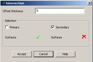
The Surface Intersection form appears where you can enter a value for an Offset intersection, if desired. A value of 0 lies on the surfaces.

·  Select the thickness of 0 and press Accept.

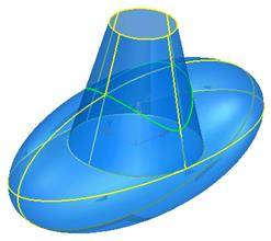
The curve/s of intersection are now calculated, and are displayed.

Any curve lying on a surface can be used to limit (trim0 a surface. The intersect command is only one way of generating a curve on a surface.

·  De-select the surfaces and select the composite curve.

·  Select Limit and then select the cone.

·  Select Next solution.

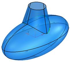
The cone is now trimmed to the composite curve. The scaled sphere is still complete and this needs to be limited to the cone

·  De-select the surfaces and select the composite curve.

·  Select Limit and then select the scaled sphere.

·  Select Next solution.

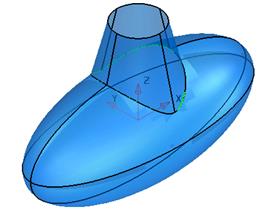
The scaled sphere now has a hole in.

·  Select and Blank the composite curve.

·  Create a plane at 0 0 32 with a length of 20 and width of 20 and a y twist of –20.

·  Limit the plane with the cone to produce a sloped top.

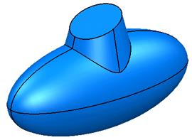
The model is complete.

·  Select File è Close and select Yes to losing Changes.