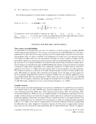
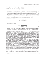





estimation purposes it is often useful to reparametrize the logistic function (2) as
|
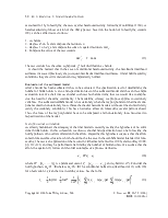
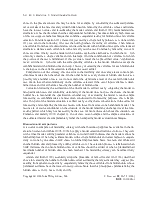
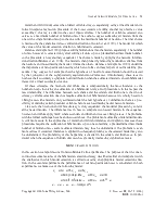
F(g i (wi¢xt - ci )) = (1+ e-g i (wi t¢x -ci ) )-1 where gi > 0, i = 1, . . . , h, and ||wi|| = 1 with |
(4) |
q
![]() wi1 = 1- Âwij2 > 0, i = 1,..., h (5)
wi1 = 1- Âwij2 > 0, i = 1,..., h (5)
j=2
The parameter vector y of model (1) becomes y = [a¢, l1, . . . , lh, g1, . . . , gh, w12, . . . , w1q, . . . , wh2, . . . , whq, c1, . . . , ch]¢. In this case the first two identifying restrictions discussed above can be defined as, first, c1 £ . . . £ ch or l1 ≥ . . . ≥ lh and, second, gi > 0, i = 1, . . ., h.
As mentioned in the Introduction, our aim is to construct a coherent strategy for building AR-NN models using statistical inference. The structure or architecture of an AR-NN model has to be determined from the data. We call this stage specification of the model, and it involves two sets of decision problems. First, the lags or variables to be included in the model have to be selected. Second, the number of hidden units has to be determined. Choosing the correct number of hidden units is particularly important as selecting too many neurons yields an unidentified model. In this work, the lag structure or the variables included in the model are determined using well-known variable selection techniques. The specification stage of NN modelling also requires estimation because we suggest choosing the hidden units sequentially. After estimating a model with h hidden units we shall test it against the one with h + 1 hidden units and continue until the first acceptance of a null hypothesis. What follows thereafter is evaluation of the final estimated model to check if the final model is adequate. NN models are typically only evaluated out-of-sample, but in this paper we also suggest the use of in-sample misspecification tests for the purpose. Similar tests are routinely applied in evaluating STAR models (Eitrheim and Teräsvirta, 1996), and in this work we adapt them to the AR-NN models. All this requires consistency and asymptotic normality for the estimators of parameters of the AR-NN model, conditions for which can be found in Trapletti et al. (2000).
The first step in our model specification is to choose the variables for the model from a set of potential variables (lags in the pure AR-NN case). Several nonparametric variable selection techniques exist (Tschernig and Yang, 2000; Vieu, 1995; Tjøstheim and Auestad, 1994; Yao and Tong, 1994; Auestad and Tjøstheim, 1990), but they are computationally very demanding, in particular when the number of observations is not small. In this paper variable selection is carried out by linearizing the model and applying well-known techniques of linear variable selection to this approximation. This keeps computational cost to a minimum. For this purpose we adopt the simple procedure proposed in Rech et al. (2001). Their idea is to approximate the stationary nonlinear model by a polynomial of sufficiently high order. Adapted to the present situation, the first step is to approximate function G(xt; y) in (1) by a general kth-order polynomial. By the Stone–Weierstrass theorem, the approximation can be made arbitrarily accurate if some mild conditions, such as the parameter space y being compact, are imposed on function G(xt; y). Thus the AR-NN model, itself a universal approximator, is approximated by another function. This yields
q q q q
G(xt;y) = p ¢x˜ t + ÂÂq j j1 2 xj t1, xj2,t + ... + Â Â... q j1...jk xj t1, ... xj tk , + R(xt;y) (6)
j1=1 j2 1= j j1=1 jk = jk-1
where R(xt; y) is the approximation error that can be made negligible by choosing k sufficiently high. The q’s are parameters, and p Œ ˙q+1 is a vector of parameters. The linear form of the approximation is independent of the number of hidden units in (1).
In equation (6), every product of variables involving at least one redundant variable has the coefficient zero. The idea is to sort out the redundant variables by using this property of (6). In order to do that, we first regress yt on all variables on the right-hand side of equation (6) assuming R(xt; y) and compute the value of a model selection criterion (MSC), AIC or SBIC for example. After doing that, we remove one variable from the original model and regress yt on all the remaining terms in the corresponding polynomial and again compute the value of the MSC. This procedure is repeated by omitting each variable in turn
Уважаемый посетитель!
Чтобы распечатать файл, скачайте его (в формате Word).
Ссылка на скачивание - внизу страницы.