Probability Distributions, Trading Strategies and Leverage: An Application of Gaussian Mixture Models

define the inverse widths of the Gaussian distributions a_i       are the mixing coefficients, with Âa_i =1

t

i           is the number of applied Gaussian mixture distributions j    is the number of applied network weights w_j k    is the number of applied network weights u_jk

2

                                                                        Gaussian distribution: Gb i (yt - mi ) =    expÁÊ - bi ◊ (yt - mi ) ˆ˜ (15) Ë   2       ¯

                                                 with m_i ( )x := Â Âw S_ij ^Ê u x_{jk k} ^ˆ ,

Ë         ¯ j            k

, b_i > 0, a_i ≥ 0, Âa_i =1

i

Sigmoid function:(16)

      Linear function:                            a G_{i bi} [y - m_i (x)]                                                 (17)

Working principle of a GM network

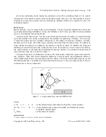
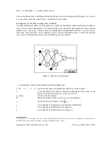
The purpose of the GM network is to mix the Gaussian distributions of the second hidden layer (Glayer) in order to model the density distribution of y_t. The width of the distributions is adapted to the whole set of training data while the locations of the distribution centres depend on the actual input data x_t and y_t. To minimize the cost function, the weights u_jk and w_ij, determining the location of the centres (m_t), have to be adapted in such a way that the distance between y_t and m_t is minimal. In doing so, the centres of the distribution are close to y_t and therefore the likelihood and with it the value of the cost function are high. See Figure 5.

Figure 5. Working principles of the GM model

Interpretation of the GM network weights

To get a better understanding of the role of the different weight groups of the network, we describe their meaning with the help of the Bayesian learning framework.

Starting with the mixing coefficients a_i, it can be interpreted as the probability that a data point has been generated from the Gaussian distribution i of the mixture. The weight is also called prior probability:

                                                       P i( ) = a_i  with  Âi a_i =1and a_i ≥ 0                                      (18)

After observing a data point (y_t,x_t), the additional information is used to update the prior probability to the posterior probability that the data point is generated from the ith component conditioned on the additional information of the actual observation (y_t,x_t):

                                                                     P i y(_t, x_t, q) = p_i (t)                                                 (19)

The relationship between both probabilities is given through Bayes’ rule:

P i y( t, xt, q) = P iq P y x i q( P y x)( (_t t_t, qt, ,) ) fi pi (t) = ati ◊Gbi (yt - mi (xt; w)) (20) Âa G_{i bi} [y - m_i (x_t; w)]

i=1

where G_bi(y_t - m_i(x_t;w)) = P(y_t|x_t,i,q) and the distribution of y_t is given by our model output P y x q(_tt, ) ⁼ Âa G_{i bi} [y - m_i (x)].

i

Update equations

It is possible to update the parameters of the GM model by gradient descent, as was done with the feedforward network. However this algorithm, due to the architectural complexity of the GM net, is very time-consuming. The update equations for a faster learning algorithm, namely the Expectation Maximization Algorithm (including the application of the Bayesian Evidence Scheme for Regularization)^[13] are more complex and are therefore presented in the Appendix.

Empirical results

Initial tests of the GM model with artificial data show that the GM is able to accurately model multimodality in the probability distributions. The data set contained four data points (x, y) where the input value x was always the same while the output value y differed. Figure 6 shows the four resulting probability distributions^[14] for the target value based on the input values of the training data. As can be seen, the GM model successfully mixed its Gaussian distributions to model the multimodality of the training data.

In order to apply the GM model to the EUR/USD return time series, we have to optimize its parameters as well as the stopping point^[15] on the test data set, which is the same data set already used with the MLP network.

Since the training process of neural networks starts with the random initialization of their weights, each network will come up with a similar but different result. To minimize the variance of the network forecasts we have split our initial investment capital equally amongst 30 identical (except

Figure 6. Probability distributions with multimodality Table VI. Parameter set of the GM model

the initial weights) GM models. The result is therefore the average result of a committee of 30 members.

We have applied many different parameter combinations (number of nodes for both hidden layers, number of iteration steps and range of possible values for the weight initialization at the beginning of the training process) to the test data set. The one we have finally chosen maximized the profit (obtained on the test data set) and is shown in Table VI.

The empirical predictions for the density functions of the exchange rate, predicted one-day-ahead, are shown in Figure 7. On the right-hand side are the probability distributions of the 290 days of the validation data set (out-of-sample data) while the left-hand side shows the predicted density function of a particular point in time. As can be seen from these graphs, it seems that there is no multimodality in the EUR/USD exchange rate market, at least within the noise level present in the data.

Using the density functions to calculate the probability