Coefficients in the Cox Model. Multiple events. Predictable time-dependent covariates

Using Time Dependent Covariates and Time Dependent

Coefficients in the Cox Model

Terry Therneau                    Cindy Crowson Mayo Clinic

April 25, 2012

1      Introduction

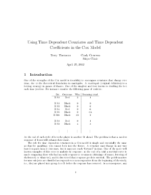
One of the strengths of the Cox model is its ability to encompass covariates that change over time, due to the theoretical foundation in martigales. A martingale (original definition) is a betting strategy in games of chance. One of the simplest and best known is doubling the bet each time you lose. For instance consider the following game of roulette:

At the end of each cycle of bets the player is another $1 ahead. The problem is that a modest sequence of losses will exhaust their stake.

The rule for time dependent covariates in a Cox model is simple and essentially the same as that for gambling: you cannot look into the future. A covariate may change in any way based on past data or outcomes, but it may not reach “forward” in time. One of the more well known examples of this error is analysis by response: at the end of a trial a survival curve is made comparing those who had an early response to treatment (shrinkage of tumor, lowering of cholesterol, or whatever), and it discovered that response predicts survival. The problem arises because subjects are classified as responders or non-responders from the beginning of the study, i.e., they are placed into group A or B before the response has occurred. As a consequence, any early deaths that occur before response can be assessed will be assigned to the non-responder group, even deaths that have nothing to do with the condition under study.

There are many variations on the error: interpolation of the values of a laboratory test linearly between observation times, removing subjects who do not finish the treatment plan, imputing the date of an adverse event midway between observation times, etc. All of these are similar to running a red light in your car: disaster is not guarranteed — but it is likely.

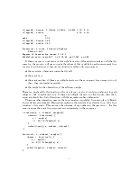
The most common way to encode time-dependent covariates is to use the (start, stop] form of the model.

> fit <- coxph(Surv(time1, time2, status) ~ age + creatinine, data=mydata)

In this data set a patient might have the following observations

In this case the variable age = age at entry to the study stays the same from line to line, while the value of creatinine varies and is treated as 1.3 over the interval (0,15], 1.5 over (15,46], etc. The intervals are open on the left and closed on the right, which means that the creatinine is taken to be 1.3 on day 15. The status variable describes whether or not each interval ended in an event.

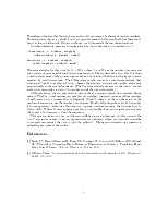
One commmon question with this data setup is whether we need to worry about correlated data, since a given subject has multiple observations. The answer is no, we do not. The reason is that this representation is simply a bookkeeping trick; the likelihood equations at any time point use only one copy of any subject, the program picks out the correct row of data at any given time. There are two exceptions to this rule, in which case the cluster variance is necessary: When subjects have multiple events.

When a subject appears in overlapping intervals. This however is almost always a data error, since it corresponds to two copies of the subject being present at the same time, e.g., they could meet themselves on the sidewalk.

2      Examples

2.1       Multiple events

Chronic granulomatous disease (CGD) is a heterogenous group of uncommon inherited disorders characterized by recurrent pyogenic infections that usually begin early in life and may lead to death in childhood. Interferon gamma is a principal macrophage-activating factor shown to partially correct the metabolic defect in phagocytes. It was hypothesized that treatment with interferon might reduce the frequency of serious infections in patients with CGD. In 1986, Genentech, Inc. conducted a randomized, double-blind, placebo-controlled trial in 128 CGD patients who received Genentech’s humanized interferon gamma (rIFN-g) or placebo three times daily for a year. The primary endpoint of the study was the time to the first serious infection. However, data were collected on all serious infections until the end of followup, which occurred before day 400 for most patients. Thirty of the 65 patients in the placebo group and 14 of the 63 patients in the rIFN-g group had at least one serious infection. The total number of infections was 56 and 20 in the placebo and treatment groups, respectively. One patient was taken off on the day of his last infection; all others have some followup after their last episode. Below are the first 10 observations, but with the listing truncatated