Improving Moving Average Trading Rules with Boosting and Statistical Learning Methods, страница 8

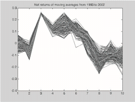
With the contingent ex ante predictive power of a single moving average having been shown, we will study the stability of returns obtained, year after year, by the different moving average rules. Figure 1 shows the annual net returns of all the 704 moving averages considered from 1993 to 2002.

As we show in Figure 1, the variability obtained by every one of the moving averages is high, producing a considerable predictive mismatching between them.

In Figure 2, where the x-axis represents every one of the 704 moving average rules, we show the mean annual net return (the oscillating line in the centre of the picture) of the moving average rules during the 10-year period considered. The three straight lines in Figure 2 correspond to the mean annual net return obtained by fi ltered Boosting strategy, the fi ltered Committee and the fi ltered Bayesian model. The top and bottom oscillating lines correspond to the confi dence intervals (m_i − 2s_i, m_i + 2s_i), where m_i and s_i are respectively the mean annual net return and the standard deviation of the annual net return of the rule i.

Figure 2 stresses several facts. The mean annual net return of every moving average rule is positive, which shows that the rules have some predictive power; the fi ltered Boosting strategy outperforms all the trading rules and the (fi ltered) Committee and (fi ltered) Bayesian (model). Also, the profi tability of the moving average rules varies every year and is volatile and a predictive mismatching is possible.

Figure 1. Annual net returns of all the 704 moving averages considered from 1993 to 2002

On the other hand, the confi dence interval corresponding to the fi ltered Boosting strategy (which was obtained as the mean annual net return ± two standard deviations of the annual net return of the rule obtained with boosting) is (−0.0530, 0.2059) ⊂ (m_i − 2s_i, m_i + 2s_i), which means that it is more profi table, less volatile and more robust that any moving average rule.

A third way of observing the variability of predictive power of moving average rules is to consider the percentile of the returns obtained by the best rule for every annual period between 1993 and 2002, as shown in Table II.

In the fi rst column of Table II the moving average with high net return during the corresponding year is presented. The next 10 columns of the table are the percentile of the annual net returns of this best rule in the distribution of the annual net returns of the universe of 704 moving averages considered. Thus:

Percentile of rule R = (Number of rules with net return ≤ rule R) / Total number of rules.

For instance, the most profi table moving average rule during 1993 was [1, 140, 0] but it was in the percentile 47.22 in 1994 and in the percentile 72.73 in 1995, etc. The most profi table rule during 1994 was [10, 80, 10], but it was in the percentile 88.99 during 1993 and in the percentile 68.18 in 1995, and so on.

Observe that in several of the columns in Table II there are several moving averages in the percentile 100. This means that there are several moving averages with the same maximum net returns during this year.

Consequently, Figures 1 and 2 and Tables I and II suggest a contingent predictive power for moving averages, that is, its capacity for obtaining net positive returns is time varying. Therefore

Figure 2. Mean annual net return (wiggly line in the centre of the picture) of every one of the 704 moving average rules during the 10-year period considered. The straight lines correspond to the mean annual net return which belongs to the fi ltered Boosting strategy (bold line), the fi ltered Committee strategy (dotted line) and the fi ltered Bayesian strategy (thin line). The top and bottom wiggly lines correspond to the confi dence intervals (m_i− 2s_i, m_i+ 2s_i) where m_i and s_i are, respectively, the mean annual net return and the standard deviation of the annual net return of rule i