Neural network linear forecasts for stock returns Angelos Kanas, страница 3

ADF is the augmented Dickey–Fuller test for the stationarity of the return series. The critical value (5%) is −2.86. This test indicates that all returns series are stationary, i.e. I(0). ^a Deviation from normality.

3. EMPIRICAL MODELS FOR STOCK RETURNS

3.1. An artificial neural network model for stock returns

An ANN model represents an attempt to emulate certain features of the way in which the brain processes information. ANN models have received considerable attention as a useful vehicle for forecasting financial variables (Swanson and White, 1995). An important feature of ANNs is that they are nonparametric models and, therefore, are appropriate for our purpose, as we do not rely on a specific functional form between stock returns, dividends and trading volumes. The specific type of ANN employed in this study is the multilayer perceptron (MLP).¹ The architecture of the MLPs trained includes one hidden layer and six hidden units. Such an MLP is denoted as MLP(1, 6). The output variable is the monthly aggregate (i.e. index) stock returns. The input variables in the input layer include the lagged percentage change of trading volume (denoted by X1) and the lagged percentage change of dividends (denoted by X2). We also set a third input variable X3, which takes the value of 1 and plays the role of a constant in a regression setting. Moreover, a link was introduced between the input variables and the output variables. As there is no reliable method of specifying the optimal number of hidden layers, we specified one hidden layer on the basis of White’s (1992) conclusion that single hidden layer MLPs do possess the universal approximation property, namely they can approximate any nonlinear function to an arbitrary degree of accuracy with a suitable number of hidden units. Moreover, as mentioned in Adya and Collopy (1998), 67% of the studies which carried out sensitivity analysis to determine the optimal number of hidden layers found that one hidden layer is generally effective in capturing nonlinear structures.

The pictorial representation of the MLP(1, 6)’s architecture employed is given in Figure 1.² The algebraic expression for the MLP(1, 6) pictured in Figure 1 is given by Equation (1), where the subscripts t from the output and input variables are suppressed to ease the exposition. Thus

                     y= a_jx_j+ b_if c_j,ix_j,                   j=1, 2       and       i=1, 2, . . . , 6                                                       (1)

                  j                    i               j

where f( . ) is the activation logistic cumulative distribution function,³ a_j are the weights for the direct signals from each of the two input variables to the output variable, b_j is the weight for the signal from each of the six hidden units to the output variable, and c_j,i are the weights for the signals from each of the two input variables to the hidden units. The logistic function is used as the activation function in order to enhance the nonlinearity of the model.

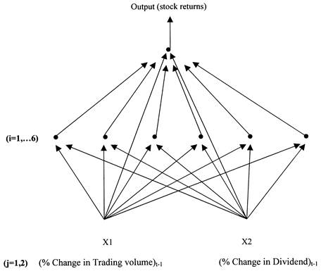
Figure 1. An MLP(1, 6) for stock returns.

The network interpretation of Figure 1 and Equation (1) is as follows. Input variables, X1 and X2, send signals to each of the hidden units. The signals from the jth input unit to the ith hidden unit is weighted by some weight denoted by c_j,i before it reaches the hidden unit number i. All signals arriving at the hidden units are first summed and then converted to a hidden unit activation by the operation of the hidden unit activation function f( . ). The next layer operates similarly with connections sent over to the output variable. As before, these signals are attenuated or amplified by weights, b_i and summed. Also, signals are sent directly from the input variables to the output variable with weight a_j. The latter signals effectively constitute the linear part of this MLP model. So, the MLP model given by Equation (1) nests the simple linear regression model and collapses to a linear model with the same explanatory variables if one sets b_i=0, or if the activation function f( . ) becomes the identity function [i.e. f(u)=u]. The nesting of the linear model within the MLP in Equation (1) ensures that the MLP will perform in-sample at least as well as the linear model.