Приближенное вычисление определенных интегралов. Методы прямоугольников и метод Симпсона

кафедра 304

Домашнее задание

по предмету «Численные методы»

по теме: «Приближенное вычисление определенных интегралов. Методы прямоугольников и метод Симпсона»

Выполнила студентка 325 гр.

Старцева А. В.

Проверила  ст. преподаватель каф. 304

Яровая О. В.

______________________

 NUMERICAL INTEGRATION

Theoretical information

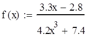
Integral of the form  in many cases it is impossible to find. For example:

·  function can not be integrated

·  function is given by the table

·  function is given by a graph

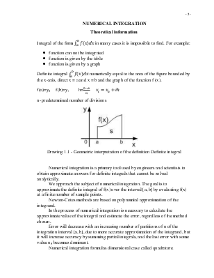
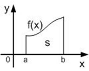
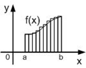
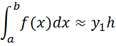
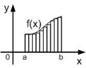
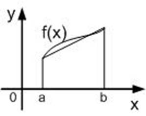
Definite integral  numerically equal to the area of ​​the figure bounded by the x-axis, direct x = a and x = b and the graph of the function f (x).

f(a)=y₀     f(b)=y₁        h=    

n- predetermined number of divisions

Drawing 1.1 - Geometric interpretation of the definition Definite integral

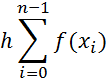
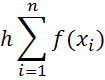
Numerical integration is a primary tool used by engineers and scientists to obtain approximate answers for definite integrals that cannot be solved analytically.
          We approach the subject of numerical integration. The goal is to approximate the definite integral of f(x) over the interval [a, b] by evaluating f(x) at a finite number of sample points.
          Newton-Cotes methods are based on polynomial approximation of the integrand.
          In the process of numerical integration is necessary to calculate the approximate value of the integral and estimate the error, regardless of the method chosen.
          Error will decrease with an increasing number of partitions of n of the integration interval [a, b], due to more accurate approximation of the integrand, but it will increase accuracy by summing partial integrals, and the last error with some value n₀ becomes dominant.
          Numerical integration formulas dimensional case called quadrature.

The idea of ​​building the quadrature formula is to replace the integrand polynomial chosen degree. We obtain the form of a quadrature formula, depending on the degree of the polynomial.

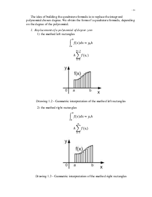
1.  Replacement of a polynomial of degree zero

1)  the method left rectangles

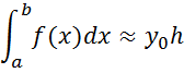
Drawing 1.2 - Geometric interpretation of the method left rectangles

2)  the method right rectangles 

Drawing 1.3 - Geometric interpretation of the method right rectangles

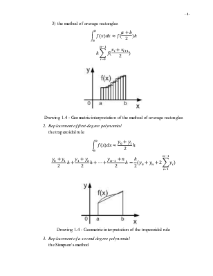
3)  the method of average rectangles

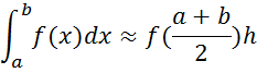
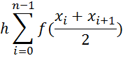
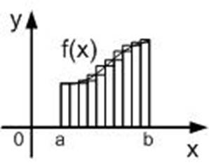
Drawing 1.4 - Geometric interpretation of the method of average rectangles

2.  Replacement of first-degree polynomial
the trapezoidal rule

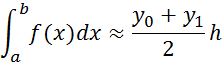
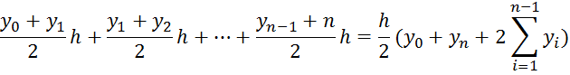
Drawing 1.4 - Geometric interpretation of the trapezoidal rule

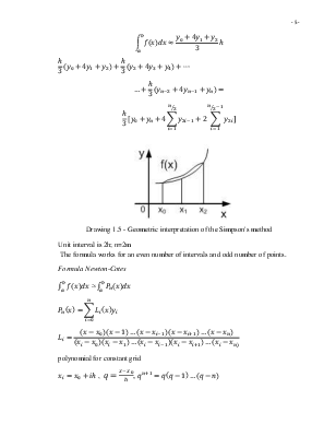
3.  Replacement of a second degree polynomial
the Simpson's method

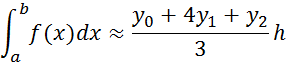
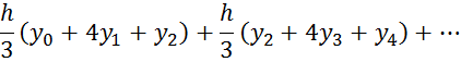
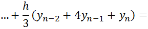
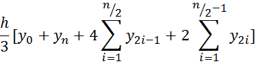
Drawing 1.5 - Geometric interpretation of the Simpson's method

Unit interval is 2h; n=2m
 The formula works for an even number of intervals and odd number of points.

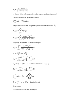
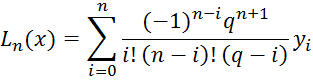
Formula Newton-Cotes

 ≈

polynomial for constant grid

 ,  ,

n- degree of the polynomial; i- number approximating polynomial

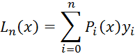
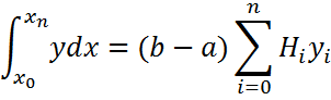
General view of the quadrature formula

 =

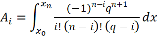
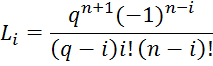
explicit form for the weighted quadrature coefficients

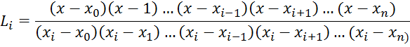
Lagrange polynomial for the uniform grid

,

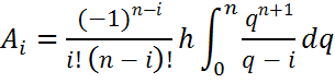
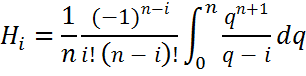
 ,  – coefficients Cotes i=(0,..n)

 , , i=(0,..,n)

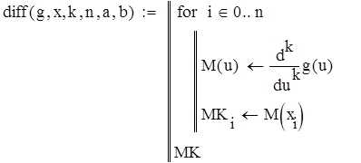
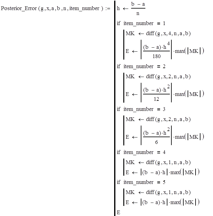
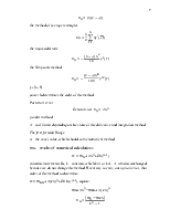
Priori error

the methods left and right rectangles

the method of average rectangles

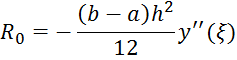
the trapezoidal rule

the Simpson's method

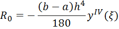
ξ є [a; b]

power h determines the order of the method

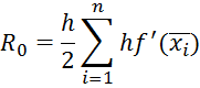
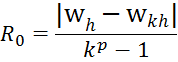
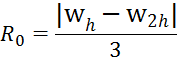
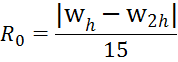
Posteriori error

General view

p-order method

A - coefficient depending on the value of the derivative and integration method

The first formula Runge

w - the exact value, which should come numerical method

 -  results of numerical calculations

w = ++O()

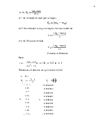
calculate increments kh, k – constant, which k>1 or k<1. A- remains unchanged, because we do not change the method. Necessary to carry out a priori error, that order of the method to determine.

w = ++O((k), equate:

+=+

 h, 2h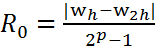  

p=1 the methods left and right rectangles

p=2 the method of average rectangles, the trapezoidal rule

p=4 the Simpson's method

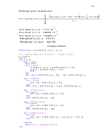
Calculate in Mathcad

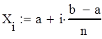
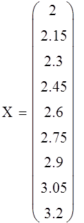
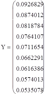
Input

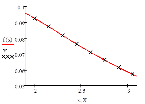
Tabulation of functions on a given interval [a,b]

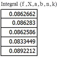
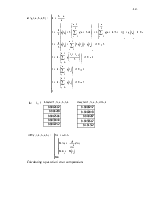
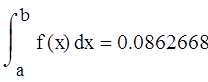
Calculation of the definite integral using the built-in

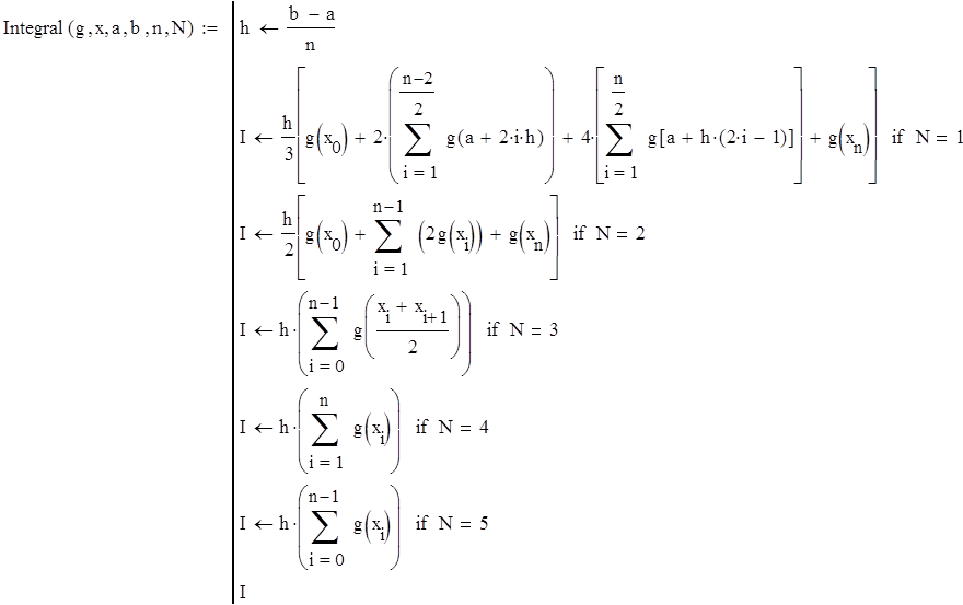
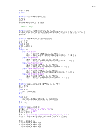
Program block that implements the calculation of the approximate value of the definite integral.

the Simpson's method

the trapezoidal rule

the method of average rectangles

the method right rectangles

the method left rectangles

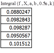
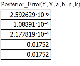
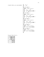
Calculating a posteriori error computation

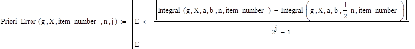
Calculating a priori calculation errors

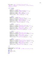
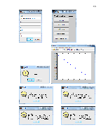
Calculate in Matlab

function res = Integral(func, str, a , b, n);

%str - methods name, a,b - distance, n - number of points

h = (b-a)/n;

Sum = 0;

 switch (str)

     case  'Simpson'

       q1=0; q2=0;

       for i = 1:n-1

            if (mod(i,2)==1) q1 = q1+myfunc(func,a + i*h);

            else q2 = q2+myfunc(func,a + i*h);

            end;       

       end;

       Sum = (h/3)*( myfunc(func,a) + 4*q1 + 2*q2 + myfunc(func,b) );

     case  'Trapezium'

        for i = 1:n-1

            Sum = Sum + myfunc(func,a + i*h);

        end;

        Sum = (h/2)*( myfunc(func,a) + 2*Sum + myfunc(func,b) );

     case  'LeftRectangles'

        for i=1:n-1

            Sum = Sum + h*myfunc(func,a + i*h);

        end;

        Sum = h*myfunc(func,a) + Sum;