Simulink for beginners

SIMULINK FOR BEGINNERS:

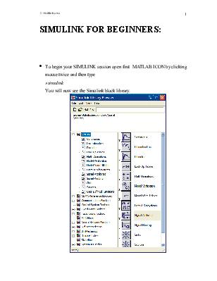
·  To begin your SIMULINK session open first  MATLAB ICON by clicking mouse twice and then type
»simulink
You will now see the Simulink block library.

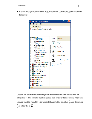
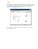
·  Browse through block libraries. E.g., if you click Continuous, you will see the following:

Observe the description of the integrator beside the block that will be used for integrator, . This operator notation comes from linear systems domain, where s is Laplace variable. Roughly, s corresponds to derivative operator, , and its inverse , to integration, .

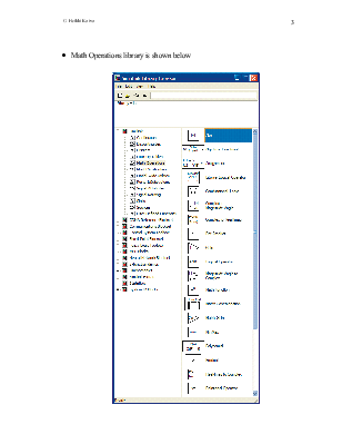
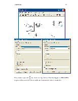
·  Math Operations library is shown below

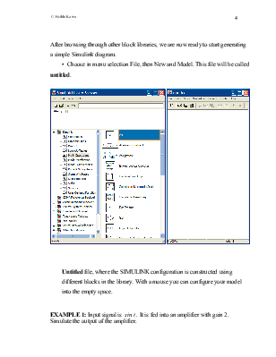
After browsing through other block libraries, we are now ready to start generating a simple Simulink diagram.

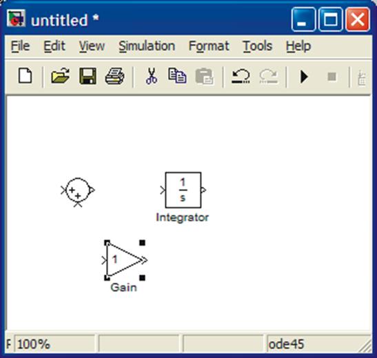
        •  Choosein menu selection File, then New and Model. This file will be called untitled.

        Untitled file, where the SIMULINK configuration is constructed using   different blocks in the library.With a mouse you can configure your model   

        into the empty space.

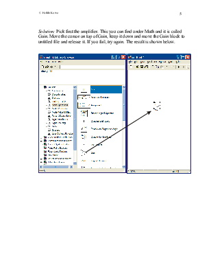
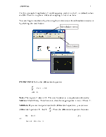
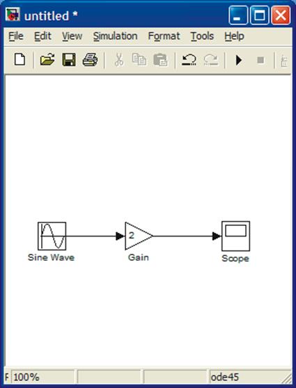
EXAMPLE 1: Input signal is  sin t . It is fed into an amplifier with gain 2. Simulate the output of the amplifier.

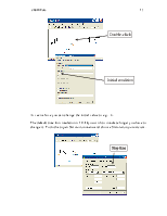
Solution: Pick first the amplifier. This you can find under Math and it is called Gain. Move the cursor on top of Gain, keep it down and move the Gain block to untitled file and release it. If you fail, try again. The result is shown below.

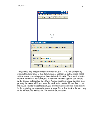
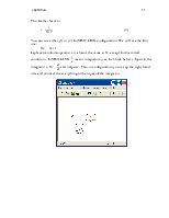
The gain has only one parameter, which has value of 1.  You can change it by moving the cursor close to 1 and clicking once and then operating as you would with any word processing system. Once finished, click OK. The numerical value inside the block will now change to 2. Next find the input signal block. This is under Sources and is called Sine Wave. Again move the cursor on top of it, keep pressing the mouse while you move the block to the untitled file and then release the mouse. In order to see the result, you need to install a sink from Sinks library. In the beginning, the easiest sink to use is scope. Move that block in the same way as the others to the untitled file. The result is shown below.

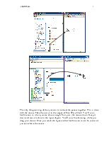
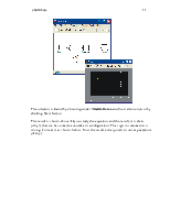
The only thing missing of the system is to connect the peaces together. This is done with the mouse. Take the cursor to the output of Sine Wave block. You’ll see a hairline cursor, when you are close enough. Now press the mouse down. Keep it down and move it close to the input of gain. You’ll see a line forming, while you drag your mouse. Once you reach the input another hairline cursor can be seen and you can release the mouse.

Your simulation system is now complete. Before simulation you should check that the parameter values in the Sine Wave block are correct. Open it by placing the cursor on top and click twice.

For this example Amplitude is 1 and frequency (rad/s) is also 1, so default values are OK. There is no phase shift and sampling is not issue here.

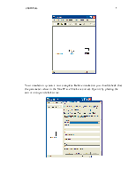
You can begin simulation by choosing Start simulation from Simulation menu or by clicking the start button.

EXERCISE 2: Solve the differential equation

Note: The input is 1 after t> 0. This can be taken as a step function from the Sources block library. Note however, that the stepping time is not t=0 but t=1.

Solution: If you are inexperienced with differential equations, you can use differential operator D.  Let  . Then the differential equation becomes

                                                                                    (1)

or

 .

This further leads to

                                                                              (2)

You can use either (1) or (2) for SIMULINK configuration. We will use the first one:

          ^.

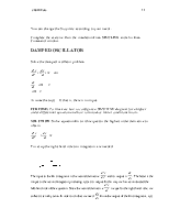
Laplace transform operator s is almost the same as D, except for the initial conditions. In SIMULINK  means integration (see the block below). Input to the integrator is and output x. Thus in configuration you set up the right hand side and connect the everything to the input of the integrator.

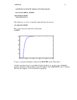
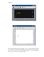
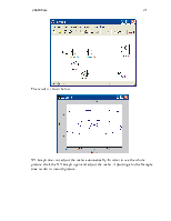
The solution is found by choosing under Simulation menu Start simulation or by clicking Start button.

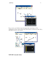
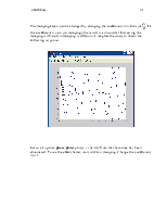
The result is shown above. If you study the equation and the result, it is clear (why?) that we have made a mistake in configuration. The sign in summation is wrong. Correct it as shown below. Now the result corresponds to our expectations (if any).

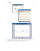
If you want to see both the input and output at the same time, use Mux (multiplexer) block, which you can find under Signals and Systems block library. Set up the system as shown below.

MATLAB Command window

Once you have defined your system in SIMULINK window, you can simulate also on the MATLAB Command window. Save your model – currently it has the name Untitled, so use that. Go to MATLAB command window and type » help sim.  The following lines will help you to understand how to simulate.

» help sim

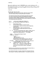
 SIM Simulate a Simulink model

    SIM('model') will simulate your Simulink model using all simulation

    parameter dialog settings including Workspace I/O options.

    The SIM command also takes the following parameters. By default

    time, state, and output are saved to the specified left hand side

    arguments unless OPTIONS overrides this. If there are no left hand side

    arguments, then the simulation parameters dialog Workspace I/O settings

    are used to specify what data to log.

    [T,X,Y]         = SIM('model',TIMESPAN,OPTIONS,UT)