Convolution Matrices for Signal Processing Applications in MATLAB
This M-book requires the Signal Processing Toolbox, version 3.0.
BASIC IDEA - TRANSFER FUNCTION
There are several discrete linear system, a.k.a. digital filter, representations used by the Signal Processing Toolbox. The most commonly used is the transfer function representation, consisting of the ratio of two polynomials
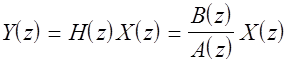
where
![]()
![]()
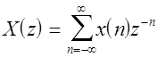
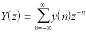
and X(z) and Y(z) are the Z-transforms of the input and output sequences x(n) and y(n) respectively:
In MATLAB the filter H(z) is represented by vectors containing the polynomial coefficients of B(z) and A(z).
Here is an example filter in the transfer function form
[b,a] = butter(5,.5)
b =
0.0528 0.2639 0.5279 0.5279 0.2639 0.0528
a =
1.0000 -0.0000 0.6334 -0.0000 0.0557 -0.0000
b contains the numerator coefficients, a contains the denominator coefficients.
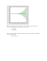
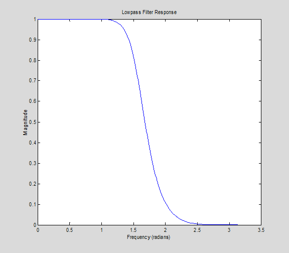
The filter's Z-transform can be computed
around the unit circle 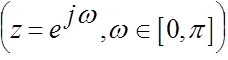 with the freqz
function
with the freqz
function
[H,w] = freqz(b,a);
plot(w,abs(H))
ylabel('Magnitude')
xlabel('Frequency (radians)')
title('Lowpass Filter Response')
CONVOLUTION MATRIX
The transfer function form is general for linear, time-invariant operators on the space of complex discrete sequences. An alternative general representation for any linear system (time-invariant or not) is an infinite dimensional matrix (a "convolution matrix").
However, infinity is not practical for implementation in MATLAB. Can a finite truncation of this matrix be useful?
IN MATLAB
Representing a system with a finite convolution matrix is ideally suited to MATLAB. Consider a system matrix C, which maps Cm to Cn (the m dimensional space of complex vectors to the n dimensional). Thus C is n-by-m. Given length n input vector x and length m output vector y, the input-output relationship of the system is
y = C*x
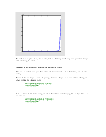
Let's compute the impulse response of our filter
h = impz(b,a)
h =
0.0528
0.2639
0.4944
0.3607
-0.0522
-0.1904
0.0055
0.1005
-0.0006
-0.0531
0.0001
0.0280
-0.0000
-0.0148
0.0000
0.0078
-0.0000
-0.0041
0.0000
0.0022
-0.0000
-0.0011
0.0000
0.0006
-0.0000
-0.0003
0.0000
0.0002
-0.0000
-0.0001
0.0000
The rows of the convolution matrix for such a time-invariant system are time shifts of the time-reversed impulse response (if the system were time varying, or adaptive, the rows would all be different in general).
The convmtx function will generate a matrix from an impulse response which, when multiplied by a signal vector, returns the convolution of the signal with the impulse response.
help convmtx
CONVMTX Convolution matrix.
CONVMTX(C,N) returns the convolution matrix for vector C.
If C is a column vector and X is a column vector of length N,
then CONVMTX(C,N)*X is the same as CONV(C,X).
If R is a row vector and X is a row vector of length N,
then X*CONVMTX(R,N) is the same as CONV(R,X).
See also CONV..
C = convmtx(h,10);
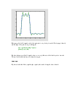
Now, take an example signal and see the equivalence of applying the convolution matrix to applying the filter in transfer function form.
format short
C1 = C(1:10,:) % keep only first ten rows (truncates output)
x = randn(10,1); % a random signal
format long e
y = filter(b,a,x)
y1 = C1*x
C1 =
Columns 1 through 7
0.0528 0 0 0 0 0 0
0.2639 0.0528 0 0 0 0 0
0.4944 0.2639 0.0528 0 0 0 0
0.3607 0.4944 0.2639 0.0528 0 0 0
-0.0522 0.3607 0.4944 0.2639 0.0528 0 0
-0.1904 -0.0522 0.3607 0.4944 0.2639 0.0528 0
0.0055 -0.1904 -0.0522 0.3607 0.4944 0.2639 0.0528
0.1005 0.0055 -0.1904 -0.0522 0.3607 0.4944 0.2639
-0.0006 0.1005 0.0055 -0.1904 -0.0522 0.3607 0.4944
-0.0531 -0.0006 0.1005 0.0055 -0.1904 -0.0522 0.3607
Columns 8 through 10
0 0 0
Уважаемый посетитель!
Чтобы распечатать файл, скачайте его (в формате Word).
Ссылка на скачивание - внизу страницы.